


“Mario Space Ship” - C, OpenGL, 10/19/04
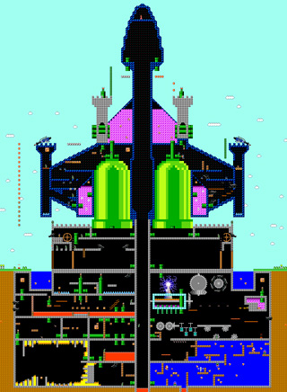 |
This is a fanciful level for the old Super Mario Bros. video game. The layout is based on one of my old drawings (1991). Note: Super Mario Bros. is copyrighted by Nintendo. In the interest of not violating any copyright laws, I have decided not to make this game available to the public. Sorry! 
|
Triangle Shape Function Interpolation - Mathematica 4.2, 5/25/06
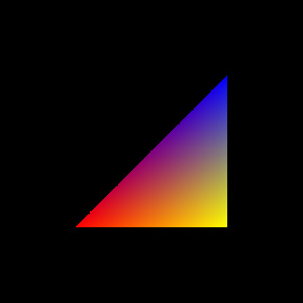 Interpolated triangles are a basic building block for generating 3D graphics. Graphics cards must be able to create these triangles very quickly. Here is some Mathematica code:
(* runtime: 2 seconds *) xIntersect[{{x1_, y1_}, {x2_, y2_}}] := If[y1 == y2, Infinity, x1 + (y - y1)(x2 - x1)/(y2 - y1)]; n = 275; image = Table[{0, 0, 0}, {n}, {n}]; xmin = ymin = 0; xmax = ymax = 1; Triangle[{p1_, p2_, p3_}, {c1_, c2_, c3_}] := Module[{}, plist = {{x1, y1}, {x2, y2}, {x3, y3}} = {p1, p2, p3}; ilist = (n - 1)(plist[[All, 2]] - ymin)/(ymax - ymin) + 1; d = Det[{{x2 - x1, y2 - y1}, {x3 - x1, y3 - y1}}];Do[y = ymin + (ymax - ymin)(i - 1)/(n - 1); {xa, xb, xc} = Map[xIntersect, Partition[Sort[plist, #1[[2]] < #2[[2]] &], 2, 1, 1]]; jlist = (n - 1)({xc, If[Abs[xb - xc] < Abs[xa - xc], xb, xa]} - xmin)/(xmax - xmin) + 1; Do[x = xmin + (xmax - xmin)(j - 1)/(n - 1); xi = Det[{{x - x1, y - y1}, {x3 - x1, y3 - y1}}]/d; eta = Det[{{x2 - x1, y2 - y1}, {x -x1, y - y1}}]/d; image[[i, j]] = (c2 - c1) xi + (c3 - c1)eta + c1, {j,Max[1, Ceiling[Min[jlist]]], Min[n, Floor[Max[jlist]]]}], {i, Max[1, Ceiling[Min[ilist]]], Min[n, Floor[Max[ilist]]]}]]; Triangle[{{0.25, 0.25}, {0.75, 0.25}, {0.75, 0.75}}, {{1, 0, 0}, {1, 1, 0}, {0, 0, 1}}]; Show[Graphics[RasterArray[Map[RGBColor @@ Map[Max[0, Min[1, #]] &, #] &, image, {2}]], AspectRatio -> Automatic]] |
3D Graphics - Mathematica 4.2, 5/25/06
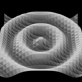
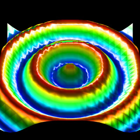 Here is some Mathematica code to demonstrate 3D graphics. A perspective projection is applied to the triangles and Phong shading is used to interpolate the surface normals across each triangle. The simplest method is the Painter’s Algorithm which draws all the polygons in the order they overlap. However, this does not account for intersecting triangles. An improved method, called Z-buffering keeps track of the depth. This method is used by OpenGL and it is usually fast enough for real-time graphics. See also my Mathematica code for a very simple ray tracer.
(* runtime: 16 seconds *) Normalize[x_] := x/Sqrt[x.x]; camloc = {0, 4, 4}; camangle = Pi/9; theta = Pi/4; Rcam = {{-1,0, 0}, {0, -Cos[theta],Sin[theta]}, {0, Sin[theta], Cos[theta]}}; {ex, ey, ez} = {0, 0, Cot[camangle/2]}; PerspectiveProjection[p_] := Module[{}, {x, y, z} = Rcam.(p - camloc); {ex - x, ey - y}ez/z]; n = 26; f := 0.125Cos[4Pi Sqrt[x^2 + y^2]]; Clear[x, y]; grad = {-D[f, x], -D[f, y], 1}; nodes = Flatten[Table[{x, y, f}, {y, -1, 1, 2/(n - 1)}, {x, -1, 1, 2/(n - 1)}], 1]; normals = Flatten[Table[Normalize[grad], {y, -1, 1, 2/(n - 1)}, {x, -1, 1, 2/(n - 1)}], 1]; colors = Flatten[Table[(1 - 8 f)/3, {y, -1, 1, 2/(n - 1)}, {x, -1, 1,2/(n - 1)}], 1]; elems = Flatten[Table[{{i, i + 1,i + n}, {i + 1, i +n + 1, i + n}} + (j - 1) n, {j, 1, n - 1}, {i, 1, n - 1}], 2]; n = 275; xmin = ymin = -1; xmax = ymax = 1; image = Table[Hue[0, 0, 0], {n}, {n}]; zbuffer = Table[-1, {n}, {n}]; xIntersect[{{x1_, y1_}, {x2_, y2_}}] := If[y1 == y2, Infinity, x1 + (y - y1)(x2 - x1)/(y2 - y1)]; Colorize[hue_, x_] := Hue[hue, Min[1, Max[0, 2(1 - x)]], Min[1, Max[0, 2x]]]; Triangle[{p1_, p2_, p3_}, {c1_, c2_, c3_}, {n1_, n2_, n3_}] := Module[{}, {{x1, y1}, {x2, y2}, {x3, y3}} = Map[PerspectiveProjection, {p1, p2, p3}]; d = Det[{{x2 - x1, y2 - y1}, {x3 - x1, y3 - y1}}]; If[d != 0, ilist = (n - 1)({y1, y2,y3} - ymin)/(ymax - ymin) + 1; n0 = Normalize[Cross[p2 - p1, p3 - p1]]; Do[y = ymin + (ymax - ymin)(i - 1)/(n - 1); {xa, xb, xc} = Map[xIntersect, Partition[Sort[{{x1, y1}, {x2,y2}, {x3, y3}}, #1[[2]] < #2[[2]] &], 2, 1, 1]]; jlist = (n - 1)({xc, If[Abs[xb - xc] < Abs[xa - xc], xb, xa]} - xmin)/(xmax - xmin) + 1; Do[x = xmin + (xmax - xmin)(j - 1)/(n - 1); xi = Det[{{x - x1, y - y1}, {x3 - x1, y3 - y1}}]/d; eta = Det[{{x2 - x1, y2 - y1}, {x - x1, y - y1}}]/d; {X, Y, z} = p3 + (p2 - p1)xi + (p3 - p1)eta;If[z > zbuffer[[i, j]], zbuffer[[i, j]] = z; lightdir = Normalize[{0, 0, 1} - {X, Y, z}]; normal = n1 + (n2 - n1) xi + (n3 - n1) eta; reflect = Normalize[2(normal.lightdir) normal -lightdir]; specular = reflect.lightdir; image[[i, j]] = Colorize[c1 + (c2 - c1) xi + (c3 - c1)eta, 0.4Max[0, normal.lightdir] + 0.6specular^10]], {j, Max[1, Ceiling[Min[jlist]]], Min[n, Floor[Max[jlist]]]}], {i, Max[1, Ceiling[Min[ilist]]], Min[n, Floor[Max[ilist]]]}]]]; Scan[Triangle[nodes[[#]], colors[[#]], normals[[#]]] &, elems]; ListDensityPlot[zbuffer, Mesh -> False, Frame -> False] Show[Graphics[RasterArray[image], AspectRatio -> 1]] |
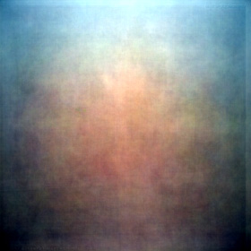
Image Deconvolution - Mathematica 4.2, 3/10/06
 Here is an amazing technique for focusing a blurry image. In order for this technique to work, the exact blurring function must be known. This technique can also be used for generating beautiful periodic textures. Here is some Mathematica code:
(* runtime: 50 seconds *) image = Import["C:/GrayPicture.jpg"][[1, 1]]; n = Length[image]; dx = 2.0/n; blurfunction = Fourier[Table[Exp[-(x^2 + y^2)/0.01^2], {y, -1, 1 - dx, dx}, {x, -1, 1 - dx, dx}]]^2; blurryimage = Re[InverseFourier[Fourier[image]blurfunction]]; ListDensityPlot[blurryimage, Mesh -> False, Frame -> False]; restoredimage = Re[InverseFourier[Fourier[blurryimage]/blurfunction]]; ListDensityPlot[restoredimage, Mesh -> False, Frame -> False] Link: Hubble telescope’s optical correction - M100 Galaxy before and after |
Delaunay Triangulation - Mathematica 4.2, 5/5/09
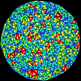 Delaunay triangulation is useful for mesh generation. The dual of a Delaunay triangulation is a Voronoi diagram. Here is some Mathematica code:
(* runtime: 1.4 seconds *) Distance[p1_, p2_] := Sqrt[(p2 - p1).(p2 - p1)]; CircleCenter[{{x1_, y1_}, {x2_, y2_}, {x3_, y3_}}] := {x1^2(y3 - y2) + x2^2(y1 - y3) + x3^2(y2 - y1) - (y3 - y2)(y1 - y3)(y2 - y1), y1^2(x2 - x3) + y2^2(x3 - x1) + y3^2(x1 - x2) + (x3 - x2)(x1 - x3)(x2 - x1)}/(2(x1(y3 - y2) + x2(y1 - y3) + x3(y2 - y1))); Triangulate[nodes_] := Module[{n = Length[nodes], p1 = Table[Min[nodes[[All, i]]], {i, 1, 2}], p2 = Table[Max[nodes[[All, i]]], {i, 1, 2}]}, nodes2 = Join[nodes, Map[(p1 + p2)/2 +Max[p2 - p1] # &, {{-20, -1}, {0, 20}, {20, -1}}]]; elems = n + {{1, 2, 3}}; Do[p = nodes[[i]]; edges = elems2 = {}; Scan[({i1, i2, i3} = #; p0 = CircleCenter[nodes2[[#]]]; If[Distance[p0,p] < Distance[p0, nodes2[[i1]]], edges = Join[edges, {{i1, i2}, {i2, i3}, {i3, i1}}], elems2 = Append[elems2, #]]) &, elems]; elems = elems2; Do[e = edges[[j]]; elist = Delete[edges, j]; If[! (MemberQ[elist, e] || MemberQ[elist, Reverse[e]]), elems = Append[elems, Append[e, i]]], {j, 1, Length[edges]}], {i, 1, n}]; Select[elems, Max[#] <= n &]]; SeedRandom[0]; nodes = Table[Random[], {100}, {2}]; elems = Triangulate[nodes]; Show[Graphics[Map[{Hue[Random[]], Polygon[nodes[[#]]]} &, elems], AspectRatio -> Automatic]] Mathematica’s ComputationalGeometry package can also be used for Delaunay triangulation: (* runtime: 0.8 second *) << DiscreteMath`ComputationalGeometry`; SeedRandom[0]; nodes = Table[Random[], {100}, {2}]; PlanarGraphPlot[nodes] Link: explanation - by Paul Bourke |
Convex Hull - Mathematica 4.2, 3/23/10
 The convex hull for a set of 2D points is the smallest possible convex polygon that can enclose those points. An easy method for finding the convex hull is the Graham Scan algorithm. Here is some Mathematica code:
(* runtime: 0.01 second *) Angle[{x_, y_}] := If[x != 0 || y != 0, ArcTan[x, y], 0]; LeftSide[{x_, y_}, {x1_, y1_}, {x2_, y2_}] := (x - x1) (y2 - y1) < (x2 - x1) (y - y1); ConvexHull[plist0_] := Module[{n = Length[plist0], i, p0 = plist0[[1]], hull}, Do[p = plist0[[i]]; If[p[[2]] < p0[[2]], p0 = p], {i, 2, n}]; plist = Sort[plist0, Angle[#1 - p0] < Angle[#2 - p0] &]; hull = {p0, plist[[2]]}; i = 3; While[i <= n, p = plist[[i]]; If[LeftSide[p, hull[[-2]], hull[[-1]]], hull = Append[hull, p]; i++, hull = Drop[hull, -1]]]; hull]; SeedRandom[0]; plist = Table[Random[], {100}, {2}]; Show[Graphics[{Map[Point, plist], Line[ConvexHull[plist]]}, AspectRatio -> Automatic]] Mathematica’s ComputationalGeometry package can also be used to find convex hulls: (* runtime: 0.8 second *) << DiscreteMath`ComputationalGeometry`; SeedRandom[0]; nodes = Table[Random[], {100}, {2}]; PlanarGraphPlot[nodes, ConvexHull[nodes]] Link: article - by Dan Sunday |
Contour Plot - Mathematica 4.2, 6/27/07
 Here is some code demonstrating how to make a simple 2D contour plot. Mathematica has a built-in function for this, but I chose to write my own code for it. Hopefully you will find it to be useful. The image on the left is a contour plot of Perlin noise. Here is some Mathematica code:
(* runtime: 0.5 second *) x1 = y1 = -4; x2 = y2 = 4; n = 15; dx = (x2 - x1)/(n - 1); dy = (y2 - y1)/(n - 1); SeedRandom[0]; mesh = Table[Random[], {n}, {n}]; interpolate[x1_, x2_, z1_, z2_] := If[Abs[2z - z1 - z2] < Abs[z2 - z1], (x2 - x1)(z - z1)/(z2 - z1) + x1]; Show[Graphics[Table[lines = {}; Do[x = x1 + i dx; y = y1 + j dy; plist = Select[{{interpolate[x - dx, x, mesh[[i, j]], mesh[[i + 1, j]]], y - dy}, {x - dx, interpolate[y - dy, y, mesh[[i, j]], mesh[[i, j + 1]]]}, {interpolate[x - dx, x, mesh[[i, j + 1]], mesh[[i + 1, j + 1]]], y}, {x, interpolate[y - dy, y, mesh[[i + 1, j]], mesh[[i + 1, j + 1]]]}}, ! MemberQ[#, Null] &]; If[Length[plist] == 2, lines = Append[lines, Line[plist]]], {i, 1, n - 1}, {j, 1, n - 1}]; lines, {z, 0, 1, 0.1}], AspectRatio -> Automatic]] |
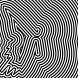
Canny Edge Detection - Mathematica 4.2, 7/7/05
 Here is a beautiful technique for finding edges. I learned this technique from Mariusz Jankowski’s Mathematica code, which uses Mathematica’s ListConvolve function.
(* runtime: 0.2 second *) image = Import["C:/GrayPicture.jpg"][[1, 1]]; A = Table[j Exp[-(j^2 + i^2)], {j, -1.0, 1.0}, {i, -1.0, 1.0}]; ListDensityPlot[Sqrt[ListConvolve[A, image]^2 + ListConvolve[Transpose[A],image]^2], Mesh -> False, Frame -> False] Here is another variation to make the image appear embossed: (* runtime: 0.1 second *) image = Import["C:/GrayPicture.jpg"][[1, 1]]; A = Table[j E^-(j^2+i^2), {j, -1.0, 1.0}, {i, -1.0, 1.0}]; ListDensityPlot[ListConvolve[A, image] + ListConvolve[Transpose[A], image], Mesh -> False, Frame -> False] Links Sobel Edge Detector - article by Bob Fisher, et al. |
Dithering - Mathematica 4.2, 9/22/08
 Here is some Mathematica code demonstrating Floyd-Steinberg Dithering:
(* runtime: 14 seconds *) image = Import["C:/GrayPicture.jpg"][[1, 1]]/255.0; ny = Length[image]; nx =Length[image[[1]]]; image2 = image; Do[c0 = image2[[i, j]]; c = Round[c0]; image2[[i, j]] = c; e = (c0 - c)/16; image2[[i + 1, j]] += 7 e; image2[[i - 1, j + 1]] += 3 e; image2[[i, j + 1]] += 5 e; image2[[i + 1, j + 1]] += e, {i, 2, ny - 1}, {j, 2, nx - 1}]; ListDensityPlot[Round[image2], Mesh -> False, Frame -> False, ImageSize -> {nx, ny}, AspectRatio -> ny/nx] Here is some Mathematica code demonstrating Ordered Dithering: (* runtime: 0.2 second *) image = Import["C:/GrayPicture.jpg"][[1, 1]]/255.0; ny = Length[image]; nx = Length[image[[1]]]; ThresholdMap = {{1, 9, 3, 11}, {13, 5, 15, 7}, {4, 12,2, 10}, {16, 8, 14, 6}}/17.0; n = Length[ThresholdMap]; ListDensityPlot[Table[Round[0.5(image[[i, j]] + ThresholdMap[[Mod[i - 1, n] + 1,Mod[j - 1, n] + 1]])], {i, 1, ny}, {j, 1, nx}], Mesh -> False, Frame -> False, ImageSize -> {nx, ny}, AspectRatio -> ny/nx] |
Blended Pictures - AutoLisp, POV-Ray 3.6.1, C++, 12/5/07; Mathematica version: 9/29/04

 The left image shows 12,629 pictures from my computer's hard drive. The right image shows what you get when you average them all together and increase the contrast (the result looks uniformly gray if you don't increase the contrast).
|
Photographic Mosaic - AndreaMosaic: 12/6/07; C++ version: 12/6/07
 This photographic mosaic was generated using Andrea Denzler's free software AndreaMosaic. I also tried to create my own version using C++, but it didn't look as nice. Click here to see an ASCII art version of this image using Unicode Chinese characters in an Excel spreadsheet.
Links Photomosaic - free software for creating irregular photographic mosaics by Chris Lomont Mosaic Creator - free software by Olej Every Second of Star Wars - picture by Jason Salavon Motion After Affect - the most amazing optical illusion I’ve ever seen Motion Illusions - by Akiyoshi Kitaoka |
Distance to a Line Segment - Mathematica 4.2, */*/09
 Here is some Mathematica code demonstrating how to find the distance to a line segment:
(* runtime: 12 seconds *) Norm[x_] := x.x; DistanceToSegment[p_, p1_, p2_] := Module[{r = Norm[p2 - p1]}, Sqrt[If[0 < (p1 - p).(p1 - p2) < r, Norm[Cross[p - p1, p2 - p1]]/r, Min[Norm[p1 -p], Norm[p2 - p]]]]]; p1 = {-1, -1, 0}; p2 = {1, 1, 0}; DensityPlot[DistanceToSegment[{x, y, 0}, p1, p2], {x, -2, 2}, {y, -2, 2}, PlotPoints -> 275, Mesh -> False, Frame -> False] |
Medial Axis - Mathematica 4.2, */*/09
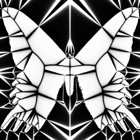 The medial axis can be useful for generating meshes. See also topological skeleton.
 |
“Torus Screensaver” - C++, OpenGL, 11/18/04
 This is an animated torus knot screensaver. The screensaver part of the code was adapted from Eric Farmer’s OpenGL screensaver template. Note: In order to run this, you might need to place glut32.dll in your Windows folder (eg: “C:/Windows/glut32.dll” or “C:/WinNT/System32/glut32.dll”). I have also included some Mathematica code and a rotatable 3D version of this surface.
 |
“Asteroids.exe” - C, OpenGL, 10/12/04
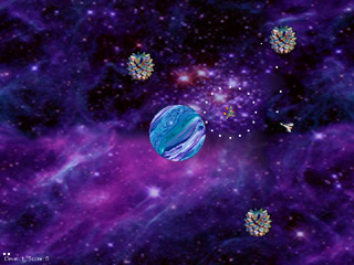 Here is a game that incorporates gravity. This game uses my original old ship design for “Aroids”, a similar game that we made at Explorer Post 340, a robotics and logic lab that I used to attend back in 1994-1997. This game has bugs but I’m too lazy to fix it. Note: In order to run this, you might need to place glut32.dll in your Windows folder (eg: “C:/Windows/glut32.dll” or “C:/WinNT/System32/glut32.dll”).
 |
“Mandelbrot.exe” - C, OpenGL, 6/8/02
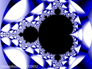 Here is a program to generate the Mandelbrot set fractal and a cubic Julia set fractal. This was my first OpenGL program. It is somewhat limited in what it can do, although the source code can easily be expanded. Note: In order to run this, you might need to place glut32.dll in your Windows folder (eg: “C:/Windows/glut32.dll” or “C:/WinNT/System32/glut32.dll”).
 |
“Test.arx” - C++, ObjectARX 2000, 11/12/04
| Here is my first AutoCAD Runtime Extension (ARX) program with source code. ARX is a C++ library for customizing AutoCAD. |
AutoLisp Programs
 Lisp (List Programming) is an interpreted language, although it can be compiled to run faster. It is also a popular language for artificial intelligence programming. I also think it’s good for programming symbolic calculators (like Mathematica). The following programs were written in AutoLisp. To run these programs, you will need access to AutoCAD:
“Tessellations.lsp” - 12/9/02, a fun program to help you create your own tessellations “Signature.vlx” - 12/20/03, a compiled Autolisp program to display the automation program signature in AutoCAD “Functions.lsp” - Here are some useful functions for finding intersection points and areas of polylines, and for testing to see if a point is inside a polyline. You can find whether a point is inside any arbitrary shape by counting the intersections from a ray outside the shape. This technique can also be extended to 3D objects, as in ray tracing. Links AfraLisp - great AutoLisp tutorials Cadalyst AutoLisp Code PLT Scheme - free, similar to Lisp |
Java Applets
“Mandelbrot” - 6/9/01, Applet along with source code to generate Mandelbrot and Julia Set fractals. This is the only Java applet on my web site at this time.
Java Links
Ken Perlin - educational computer graphics, many Java applets: Face Demo, Car, etc.
Rubik’s Cube Java Applets - 3x3, 4x4, and 5x5
Arcade Emulators: Borne d'arcade, JEmu
particle simulator - fun Java applet by Chris Laurel
Voxel - 3D Flight Simulator Java applet
Connect 4 - Java applet
Graphics Links
NeHe - great OpenGL tutorials (particles, mirrors, etc.) and OpenGL contest (my favorite is “Water Garden”)
Paul Bourke - tons of graphics information
Sulaco - impressive Delphi programs by Jan Horn, see Dynamic Cube Mapping, SAGameDev Demo, Peristalsis, Plasma Tunnel
Paul Baker - OpenGL C programs, see Cloth Simulation, Shadow Volumes, Quake 3 BSP, Bump Mapping, Render To Texture
Hugo Elias - graphics information and physics simulations
Bitmap Tutorial - how to make bitmaps, by Andreas Hartl
Other Programming Links
Microsoft Visual Studio Express Editions - free compilers from Microsoft, includes Visual C++, Visual C#, Visual J#, Visual Basic, and ASP
RoboCup - project to build robots that can beat human professional soccer players by the year 2050, see this video
Artificial Linguistic Internet Computer Entity (ALICE) - awarded “most-human” chatbot, decide for yourself, see also Turing Test
Breaking a Visual CAPTCHA - an algorithm that can break CAPTCHA tests (Completely Automated Public Turing Test to tell Computers and Humans Apart)
Play 20 Questions with Darth Vador - funny algorithm