


Minimal surfaces are surfaces that span an arbitrarily shaped boundary with minimal surface area. For example, surface tension can cause soap films to form minimal surfaces. These surfaces can be very beautiful.
Gyroid - Mathematica 4.2, POV-Ray 3.6.1, 3/25/11
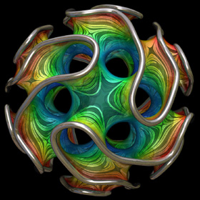

 You can purchase this as a poster, a tie, or a printed fabric pattern.
The Gyroid is a type of triply periodic minimal surface that was discovered by Alan Schoen in 1970. It can be approximated by a simple isosurface defined by cos(x)sin(y) + cos(y)sin(z) + cos(z)sin(x) = 0. The surface patterns in this image are actually artifacts that were created as a result of lowering the max_gradient parameter in POV-Ray. The colors remind me of Yellowstone's hot spring pools. Here is some Mathematica code: (* runtime: 8 seconds *) << Graphics`ContourPlot3D`; ContourPlot3D[Cos[x]Sin[y] + Cos[y]Sin[z] + Cos[z]Sin[x], {x, -5, 5}, {y, -5, 5}, {z, -5, 5}, Contours -> {0}, PlotPoints -> 6, ViewPoint -> {1, 1, 1}] and here is some POV-Ray code: // runtime: 4 seconds camera{location 10 look_at 0} light_source{10,1} isosurface{function{cos(x)*sin(y)+cos(y)*sin(z)+cos(z)*sin(x)} threshold 0 max_gradient 2 contained_by{sphere{<0,0,0>,7}} open pigment{rgb 1}} Links Gyroid Labyrinth Graph - by EPINET project Order 2 Gyroid, Order 3 Gyroid - Mathematica code for the exact parametric formula, by Matthias Weber Steel Gyroid - by Florian Sanwald Triple Gyroid Sphere - by Stijn van der Linden Gyroid - a popular 3D metal printed piece, by Bathsheba Grossman Gyroid - MathWorld article |
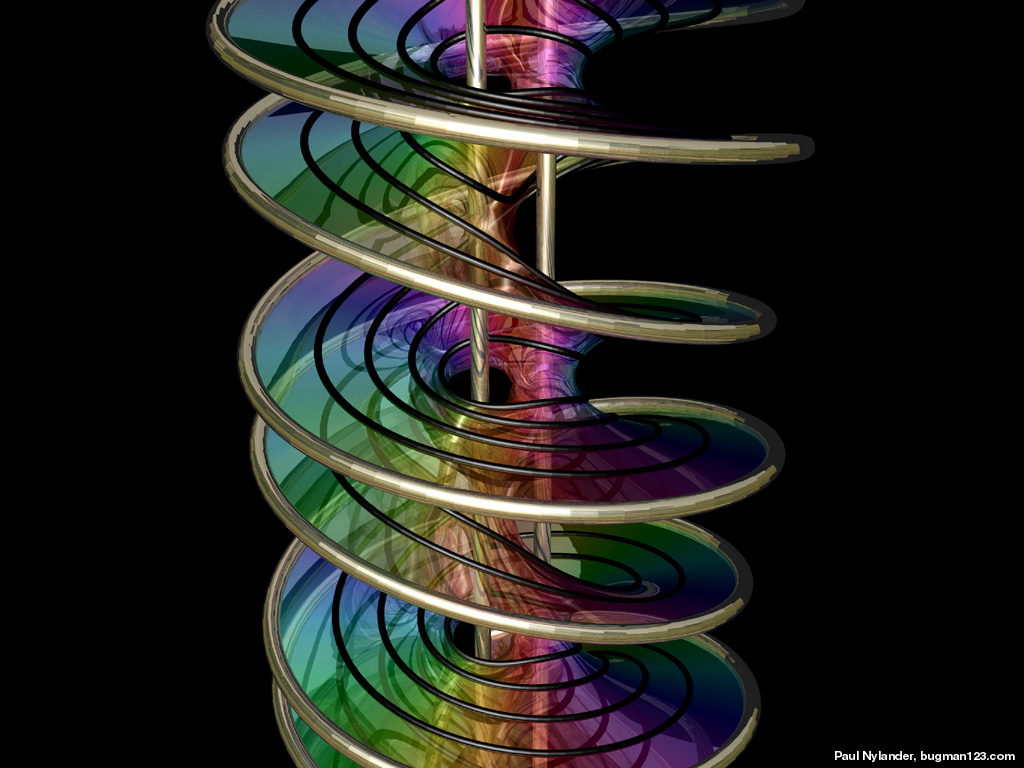
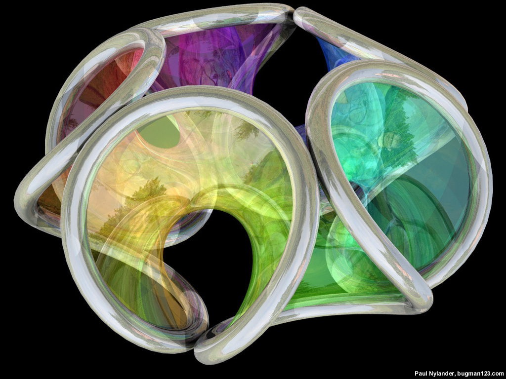
Scherk-Collins Surface - Mathematica 4.2, POV-Ray 3.6.1, old version: 7/19/06, new version: 2/10/09

 This surface can be formed by twisting and warping a singly-periodic Scherk’s minimal surface. This idea was originally attributed to Brent Collins. Technically, the surface is no longer considered exactly "minimal" after twisting but it still looks minimal (it is actually very difficult to find the exact shape for most minimal surfaces). Click here to download some POV-Ray code and here for some AutoLisp code. Here is some Mathematica code:
(* runtime: 0.3 second *) << Graphics`Master`; n = 5; r = 0.75n; Twist[{x_, y_, z_}, theta_] := {x Cos[theta] - y Sin[theta], x Sin[theta] + y Cos[theta], z}; Warp[{x_, y_, z_}, theta_] := {(x + r) Cos[theta], (x + r) Sin[theta], y}; f[z_] := Module[{t1 = Sqrt[2Cot[z]], t2 = Cot[z] + 1}, Warp[Twist[Re[{0.5xsign(Log[t1 - t2] - Log[t1 + t2])/Sqrt[2], ysign I(ArcTan[1 - t1] - ArcTan[1 + t1])/Sqrt[2], z}], 2Re[z]/n], 2Re[z]/n]]; DisplayTogether[Table[ParametricPlot3D[f[x + I y], {x, 0, n Pi}, {y, 0.001, 0.75}, PlotPoints -> {8n + 1, 5}, Compiled -> False], {xsign, -1, 1, 2}, {ysign, -1, 1, 2}]] The following Mathematica code can be used to increase the number of edges (or "branches"). This code uses some complicated functions that were adapted from Matthias Weber's Mathematica notebook: (* runtime: 1.2 seconds *) << Graphics`Shapes`; k = 4; phi = Pi(0.6/k - 0.5)/(1 - k); f[z_] := Re[NIntegrate[Evaluate[{0.5 (w^(1 - k) - w^(k - 1)), 0.5 I (w^(1 - k) + w^(k - 1)), 1}/(w^(k + 1) + w^(1 - k) - 2w Cos[k phi])], {w, 0, z}]]; alpha = Pi/k; zbeta = Exp[I Pi(phi/alpha - 0.5)]; surface = ParametricPlot3D[Re[f[Exp[I alpha/2]((1 + I zbeta Exp[r + I theta])/(I Exp[r + I theta] -zbeta))^(alpha/Pi)]], {r, 0, 4}, {theta, 0, Pi}, PlotPoints -> 10, Compiled -> False, DisplayFunction -> Identity][[1]]; z0 = f[1][[3]]; surface = {surface, AffineShape[TranslateShape[surface, {0, 0, -2z0}], {1, 1, -1}]}; surface = {surface, AffineShape[surface, {1, -1, 1}]}; surface = Table[RotateShape[surface, 2Pi i/k, 0, 0], {i, 1, k}]; dz = Pi Csc[k phi]/k; Show[Graphics3D[Table[TranslateShape[surface, {0, 0, i dz}], {i, 0, 1}]]] Links “Whirled White Web” - a beautiful snow sculpture by Brent Collins Sculpture Generator - C++ program for Scherk-Collins surfaces by Carlo Séquin |
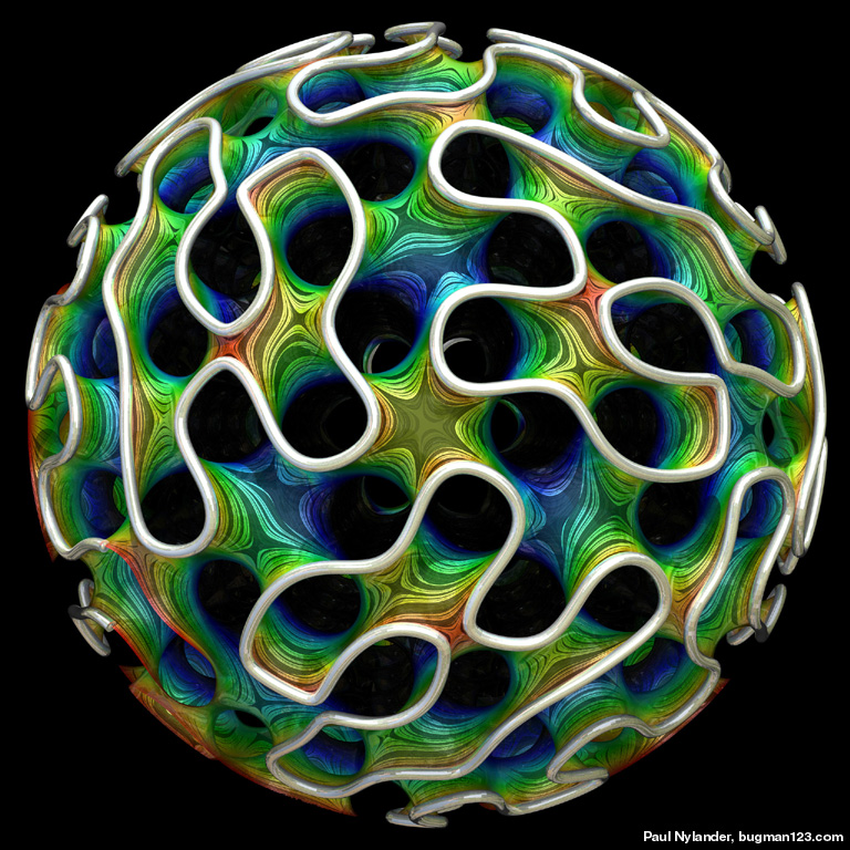
Punctured Helicoid - Mathematica 4.2, POV-Ray 3.6.1, 1/13/09
 Here is a helicoid with holes in it. This image was printed on the cover of McGraw-Hill's 2012 & 2013 Algebra1 textbooks. The following Mathematica code uses some complicated functions that were adapted from Matthias Weber's Mathematica notebook:
(* runtime: 4 seconds *) << Graphics`Shapes`; tau0 = Exp[1.23409 I]; b0 = 0.629065; theta[z_] := EllipticTheta[1, Pi z, Exp[I Pi tau0]]; r1[z_] := theta[z + 0.5 (b0 - 2) (tau0 + 1)]/theta[z + 0.5 (b0 - 1) (tau0 + 1)]; r2[z_] := theta[z - 0.5 b0 (tau0 + 1)]/theta[z - 0.5 (b0 + 1) (tau0 + 1)]; omega3[z_] := r1[z] r2[z]/(0.386191 - 0.169839 I); G[z_] := (108.37 - 62.8417 I) Exp[I Pi (b0 - 2 z + 2 tau0 + b0 tau0)]r1[z]/r2[z]; f[z0_] := Re[NIntegrate[Evaluate[{-(G[z] omega3[z] - omega3[z]/G[z] )/2, I(G[z] omega3[z] + omega3[z]/G[z] )/2, omega3[z]}], {z, tau0/2, z0}]] + {0.434156, 0, -1}; a0 = -0.409956; r0 = 2.43051; g[z_] := (EllipticF[ArcSin[(a0 + r0 E^z)/(1 - a0 E^z)], 1/r0^2]/(2EllipticF[Pi/2, 1/r0^2]) + 0.5)(1 + tau0)/2; surface = ParametricPlot3D[f[g[x + I y]], {x, -2.5, 2.5 - 0.8881}, {y, 0.001,0.999Pi}, PlotPoints -> {15, 10}, Compiled -> False, DisplayFunction -> Identity][[1]]; surface = {surface, RotateShape[surface, 0, 0, Pi]}; Show[Graphics3D[{surface, TranslateShape[surface, {0, 0, 2}]}, ViewPoint -> {1, 6, 3}]] |
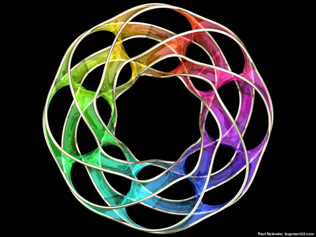
Catenoid/Helicoid - POV-Ray 3.6.1, 1/8/09
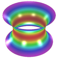
 When soap film is applied over a helical spring, it usually takes the form of a minimal surface called a helicoid. However, it is also possible for the soap film to form a different minimal surface which is a cross between a catenoid and a helicoid. The left image shows one such catenoid/helicoid that has been warped around a circle. Click here to download some POV-Ray code and here for some AutoLisp code. Here is some Mathematica code:
(* runtime: 0.6 second *) x := Sin[alpha]Cosh[v]; y := Cos[alpha]Sinh[v]; Do[ParametricPlot3D[{x Cos[u] + y Sin[u], x Sin[u] - y Cos[u], u Cos[alpha] + v Sin[alpha]}, {u, 0, 2Pi}, {v, -2.25, 2.25}, PlotPoints -> {36, 10}], {alpha, -Pi/2, Pi/2, Pi/18}]; Links Venice Museum Bridge - bridge proposal, by Eric Worcester Marina Bayfront Pedestrian Bridge - double-helix bridge in Singapore Soap Film Coil Photos - by John Oprea Soap Film Coil Photo - by the Exploratorium |
Costa’s Minimal Surface - Mathematica 4.2, POV-Ray 3.6.1, 4/3/05
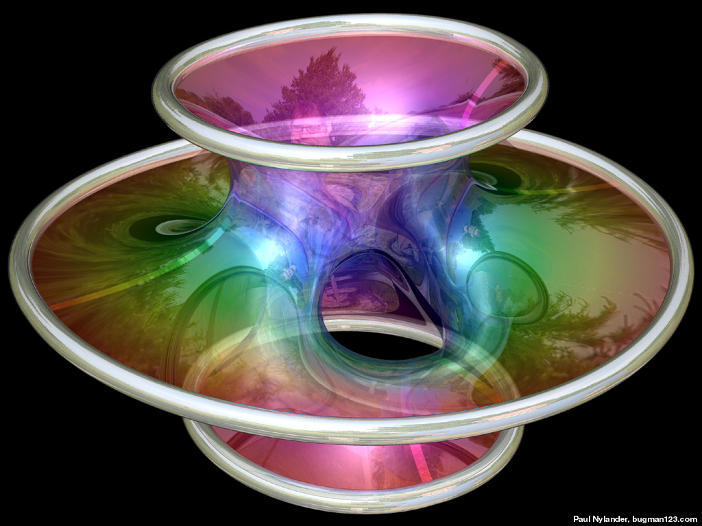
 Costa's minimal surface is a classic example of a minimal surface with holes in it, also called "handles". The number of holes is called the genus of the surface. Costa was a graduate student when he discovered this surface. They say he resolved the equation in his dreams. Here is some Mathematica code:
(* runtime: 5 seconds *) Costa[z_] := Module[{phi1 = -2 Sqrt[z] Sqrt[1 - z^2] Hypergeometric2F1[1/4, 3/2, 5/4, z^2]/Sqrt[z^2 - 1], phi2 = -(2/3) z^(3/2) Sqrt[z^2 - 1] Hypergeometric2F1[3/4, 1/2, 7/4, z^2]/Sqrt[1 - z^2]}, Re[{phi2 - phi1, I(phi1 +phi2), Log[z - 1] - Log[z + 1]}]/2]; surface = ParametricPlot3D[Costa[Sqrt[Exp[r - I theta] + 1]], {r, -3.5, 6}, {theta, -Pi, Pi}, PlotPoints -> {20, 18}, Compiled -> False][[1]]; << Graphics`Shapes`; surface = {surface, RotateShape[surface, Pi, 0, 0]}; Show[Graphics3D[{surface, RotateShape[surface, Pi/2, Pi, 0]}]] Here is another parametrization: (* runtime: 5 seconds *) c = 189.07272; e1 = 6.87519; Costa[u_, v_] := Module[{z =u + I v}, zeta = WeierstrassZeta[z, {c, 0}]; zeta1 = WeierstrassZeta[z - 1/2, {c, 0}]; zeta2 = WeierstrassZeta[z - I/2, {c, 0}]; p = WeierstrassP[z, {c, 0}]; x = Re[Pi (u + Pi/(4 e1) ) - zeta + Pi(zeta1 - zeta2)/(2 e1)]/2; y = Re[Pi (v + Pi/(4 e1)) - I(zeta + Pi(zeta1 - zeta2)/(2 e1))]/2; z = (Sqrt[2 Pi]/4)Log[Abs[(p - e1)/(p + e1)]]; {x, y, z, EdgeForm[]}]; ParametricPlot3D[Costa[u, v], {u, 0.0001, 1}, {v, 0.0001, 1}, PlotPoints -> 40, PlotRange -> {{-3.5, 3.5}, {-3.5, 3.5}, {-2, 2}},Compiled -> False] Links Topology of Costa's Minimal Surface - homotopy that continuously maps a torus into Costa's surface, by Stewart Dickson Mathematica code and minimal surface art - by Matthias Weber Alfred Gray - differential geometry gallery soap bubble light interference - by Kei Iwasaki Eva Hild - beautiful ceramic sculptures minimal surfaces with metal frames Helaman Ferguson - math sculptor, see his Costa snow sculpture |
Naturally Formed Costa’s Minimal Surface - Paint Film on 3D Printed Nylon Boundary, 2/3/14
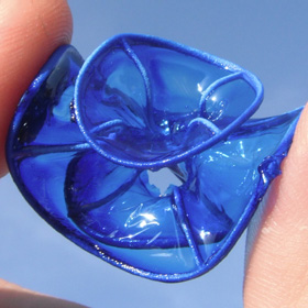 For many years, I have wanted to see if Costa’s minimal surface could be naturally formed using soap film. Here is my first attempt to accomplish this by dipping a 3D printed boundary into paint that behaves like soap film. Unfortunately, the boundary became distorted by the film's surface tension. More to come soon...
Links Making a Modified Costa Surface with Soap Film - by Andrew Bayly |
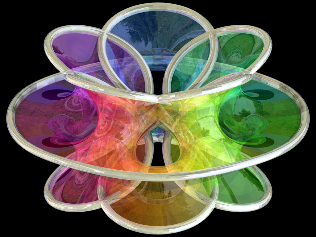
Higher Genus Costa’s Minimal Surfaces - Mathematica 4.2, POV-Ray 3.6.1, 6/28/10
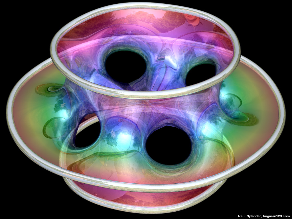
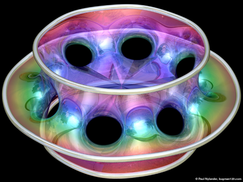
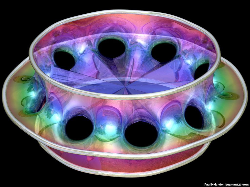 The following Mathematica code can be used to increase the number of holes. This code uses some complicated functions that were adapted from Matthias Weber's Mathematica notebook:
(* runtime: 1.2 seconds *) n = 5; psi1[z_] := n z^(1/n) Hypergeometric2F1[0.5/n, 1 + 1/n, 1 + 0.5/n, z^2]; psi2[z_] := (n/(2 n - 1)) z^(2 - 1/n) Hypergeometric2F1[1 - 0.5/n, 1 - 1/n, 2 - 0.5/n, z^2]; rho = Sqrt[4^(1/n)Gamma[1 - 0.5/n] Gamma[(n + 1)/(2 n)]/(Gamma[1 + 0.5/n] Gamma[(n - 1)/(2 n)])]; f[z_] := 0.5Re[{psi2[z]/rho - rho psi1[z], I (psi2[z]/rho + rho psi1[z]), Log[(z - 1)/(z + 1)]}]; surface = ParametricPlot3D[f[Sqrt[Exp[x + I y] + 1]], {x, -3, 6}, {y, 1.0*^-6, Pi}, PlotPoints -> {30, 15}, Compiled -> False, DisplayFunction -> Identity][[1]]; << Graphics`Shapes`; surface = {surface, RotateShape[surface,Pi/n, Pi, 0]}; surface = {surface, AffineShape[surface, {1, -1, 1}]}; Show[Graphics3D[Table[RotateShape[surface, 2Pi i/n, 0, 0], {i, 1, n}]]]; |
Triple Bubbles - Mathematica 4.2, POV-Ray 3.6.1, 7/*/10

 In order to simulate bubbles correctly, every bubble intersection must meet at exactly 120° angles. See also my Dodecaplex rendering. Here is some Mathematica code:
(* runtime: * seconds *) Links Popping Bubbles Simulation - amazing simulation, by James Sethian and Robert Saye Triple Bubbles - Mathematica notebook, uses purely geometric methods, by Wilberd van der Kallen, et. al. Double Bubbles - by John Sullivan 120 Cell Soap Bubbles - by John Sullivan |
Fourth Enneper Surface - Mathematica 4.2, POV-Ray 3.6.1, 6/4/05
 Click here to download some POV-Ray code for this image and here for some AutoLisp code. Here is some Mathematica code for the Second Enneper surface:
(* runtime: 0.5 second *) n = 3; ParametricPlot3D[{r Cos[phi] - r^(2n - 1) Cos[(2n - 1) phi]/(2n - 1), r Sin[phi] + r^(2n - 1) Sin[(2n - 1) phi]/(2n - 1), 2 r^n Cos[n phi]/n, EdgeForm[]}, {phi, 0, 2Pi}, {r, 0, 1.3}, PlotPoints -> {181, 20}, ViewPoint -> {0, 0, 1}, PlotRange -> All] Links Enneper Mathematica Notebook Enneper Snow Sculpture |
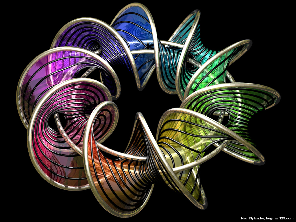
Chen-Gackstatter Minimal Surface - POV-Ray 3.6.1, 2/25/09
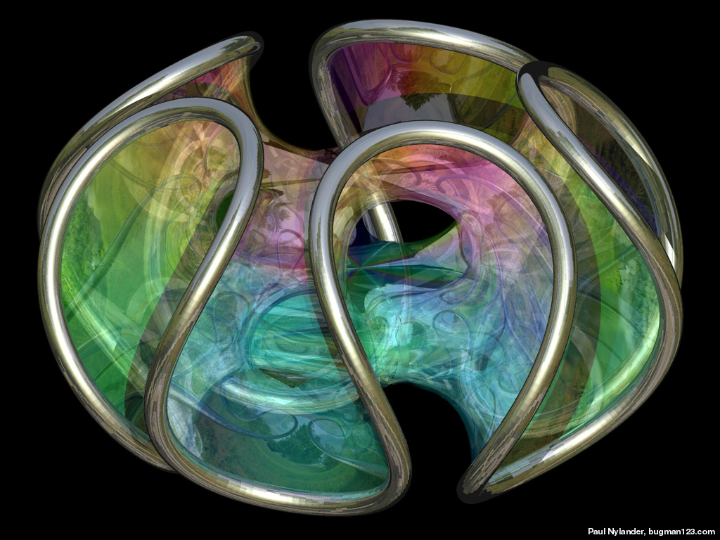 This modified Enneper surface has holes in it. The following Mathematica code uses some functions that were adapted from Matthias Weber's Mathematica notebook:
(* runtime: 0.4 second *) << Graphics`Shapes`; k = 5; n = (k - 1)/k; rho = 1.0/Sqrt[4^n Gamma[(3 - n)/2] Gamma[1 + n/2]/(Gamma[(3 +n)/2]Gamma[1 - n/2])]; phi[n_, z_] := z^(n + 1)Hypergeometric2F1[(n + 1)/2, n, (n + 3)/2, z^2]/(n + 1); f[z_] := {0.5(phi[n, z]/rho - rho phi[-n, z]), 0.5I(rho phi[-n, z] + phi[n, z]/rho), z}; surface = ParametricPlot3D[Re[f[r Exp[I theta]]], {r, 0, 2}, {theta, 1*^-6, 2Pi}, PlotPoints -> {9, 33}, Compiled -> False, DisplayFunction -> Identity][[1]]; Show[Graphics3D[Table[RotateShape[surface, 0, 0, 2Pi i/k], {i, 0, k - 1}]]] |
Giant Bubble - 3/20/05
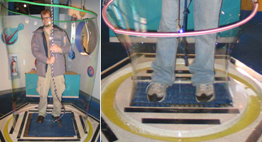
 We made these giant soap films at the Children’s Museum. Due to surface tension, the sides of these soap films would slowly shrink inward to form a minimal surface called a catenoid:
(* runtime: 4 seconds *) r := Cosh[z]; ParametricPlot3D[{r Cos[theta], r Sin[theta], z, {EdgeForm[], SurfaceColor[Hue[theta/(2Pi)]]}}, {theta, 0, 2Pi}, {z, -2,2}, Axes -> False, Boxed -> False, PlotPoints -> {73, 51}]; Bubble Links Bubble Records - impressive bubbles by Fan Yang Zubbles - colored bubbles Maarten Rutgers - uses soap films like 2D wind tunnels, see his soap film vortices and 50' soap film antibubbles - interesting Double Bubbles and Polytope Bubbles by John Sullivan nice rendering of bubbles |
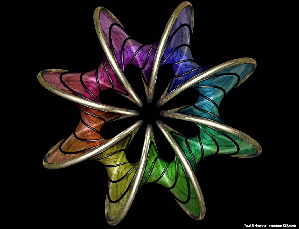
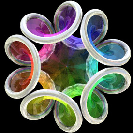
Jorge-Meeks K-Noids - POV-Ray 3.6.1, 1/16/09
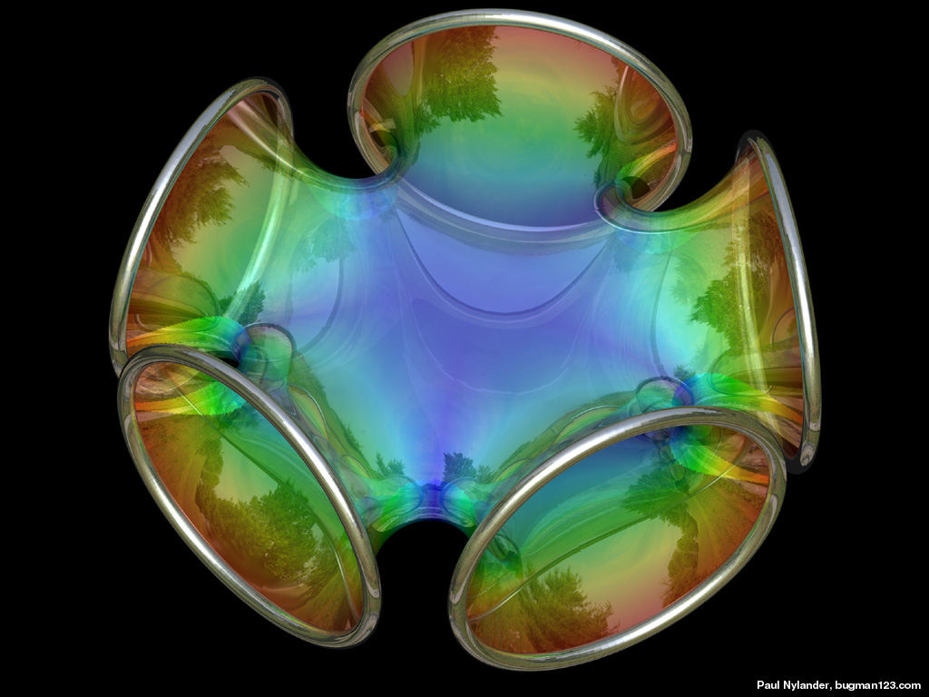
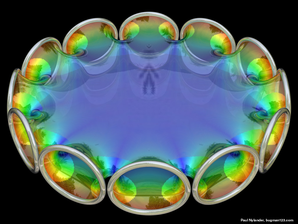 The following Mathematica code uses some functions that were adapted from Matthias Weber's Mathematica notebook:
(* runtime: 0.4 second *) << Graphics`Shapes`; k = 5; phi1[z_] := z^(k - 1) (k/(1 - z^k) - (k - 1) LerchPhi[z^k, 1, 1 - 1/k])/k^2; phi2[z_] := z(1/(1 - z^k) + (k - 1)LerchPhi[z^k, 1, 1/k]/k)/k; f[z_] := {0.5 (phi2[z] - phi1[z]), 0.5 I (phi1[z] + phi2[z]), 1/(k - k z^k)}; surface = ParametricPlot3D[Re[f[(1 + 2/(I Exp[x + I y] - 1))^(2/k)]], {x,0, Pi/2}, {y, -Pi/2, Pi/2}, PlotPoints -> {8, 16}, Compiled -> False, DisplayFunction -> Identity][[1]]; surface = {surface, AffineShape[surface, {1, -1, 1}]}; Show[Graphics3D[Table[RotateShape[surface, 0, 0, 2Pi i/k], {i, 0, k - 1}]]]; Links Mathematica notebook - by Matthias Weber Symmetric 4-Noid - at the Virtual Math Museum |
Richmond’s Minimal Surface - Mathematica 4.2, POV-Ray 3.6.1, 6/6/07
 I learned about this minimal surface from Brian Johnston’s website. Click here to download some AutoLisp code for this image. Here is some Mathematica code:
(* runtime: 2 seconds *) Richmond[n_, z_] := {-1/(2z) - z^(2n + 1)/(4n + 2), -I/(2z) + I z^(2n + 1)/(4n + 2), z^n/n}; ParametricPlot3D[Re[Richmond[5, r Exp[I theta]]], {r, 0.53, 1.187}, {theta, 0, 2Pi}, PlotPoints -> {25, 180}, Compiled -> False] |
Other Minimal Surface Links
Bubble Drawings - an interesting idea of letting bubbles and ink dry on paper, by Charlotte Sullivan
Green Void - minimal surface artwork made from large sheets, by LAVA
Discrete Minimal Surfaces - minimal surfaces with inscribed circles, by Alexander Bobenko and Tim Hoffmann