


On this page you will find some tessellations, surfaces, and other math stuff along with some basic Mathematica code.
 - POV-Ray version: 10/7/08; 3ds Max, MaxScript model: 3/15/11
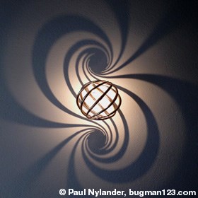
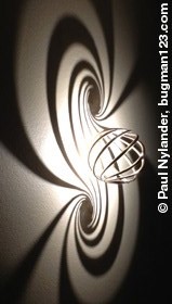
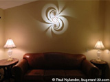
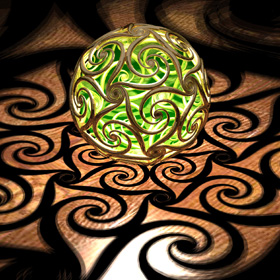
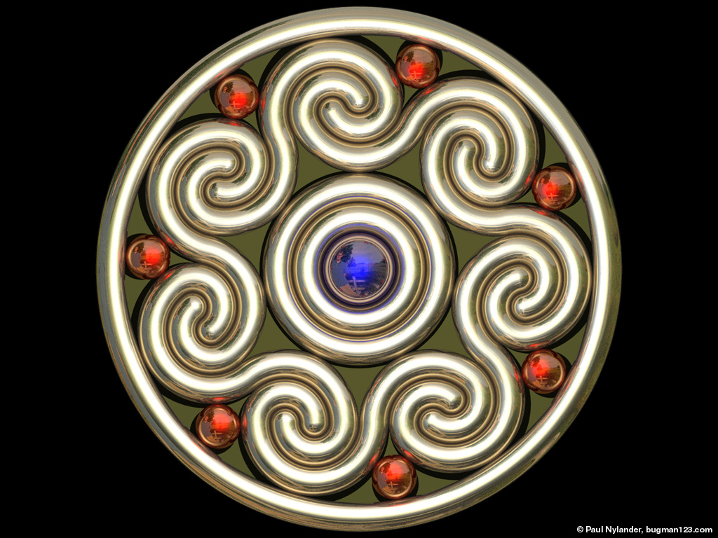
 This sconce light demonstrates how to create a double spiral by applying a light projection from one side of a loxodrome to a wall on the other side. In mathematics, we call this type of projection a stereographic projection. I finished a small 4 inch prototype on 10/10/11, and presented a large 8 inch model at the 3D Printer World Expo 2014. It received many positive responses from viewers. Click here if you would like to purchase one.
The loxodrome is a nautical term referring to the path that a ship follows on the Earth if it maintains a constant heading. For example, if a ship maintains a heading of 45° North-East, then it will spiral around the North pole as it approaches the pole, but it will never reach the North pole because it is not pointing due North. Similarly, the ship will spiral around the South pole in the opposite direction if it follows the path in reverse. |
Sand Dollar Arch - C# SolidWorks plugin, Blender, 8/4/20
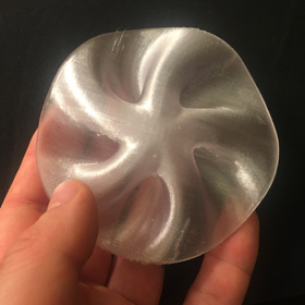
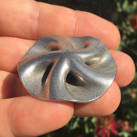
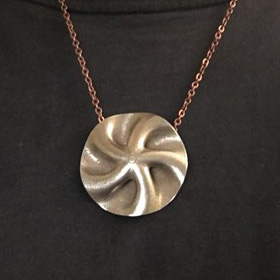 This design was inspired after my Sand Arch (which was inspired after the Jacob Hamblin Arch). It has 5 tunnels that meet at the center, and it is symetrical on both sides. If you flip it over, the tunnels become the arches and the arches become the tunnels. The model in the left photo was 3D printed in transparent PETG using my Creality3D Ender-3 Fused Deposition Modeling (FDM) 3D printer. The model in the right photo was 3D printed in Polished Bronzed-Silver Steel and it makes a nice necklace pendant. You can buy it here.
 |
Sand Arch, 5/23/17
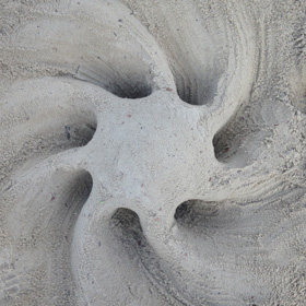
 I got inspired to make this spiraling sand arch with multiple tunnels after seeing photos of the Jacob Hamblin Arch. Click here to see a movie going through the tunnel.
 |
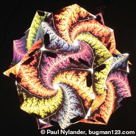
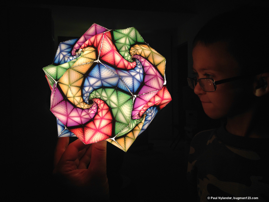
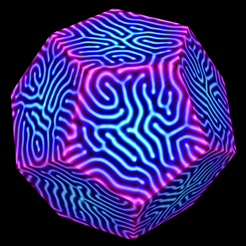
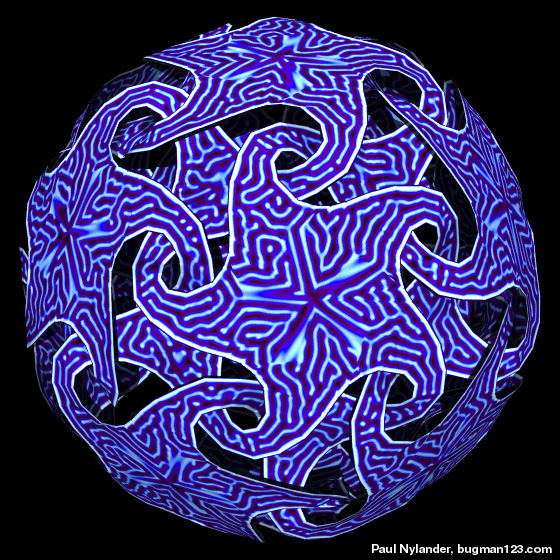
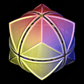
Dodeca-Spidroball - POV-Ray 3.6.1, 7/29/10
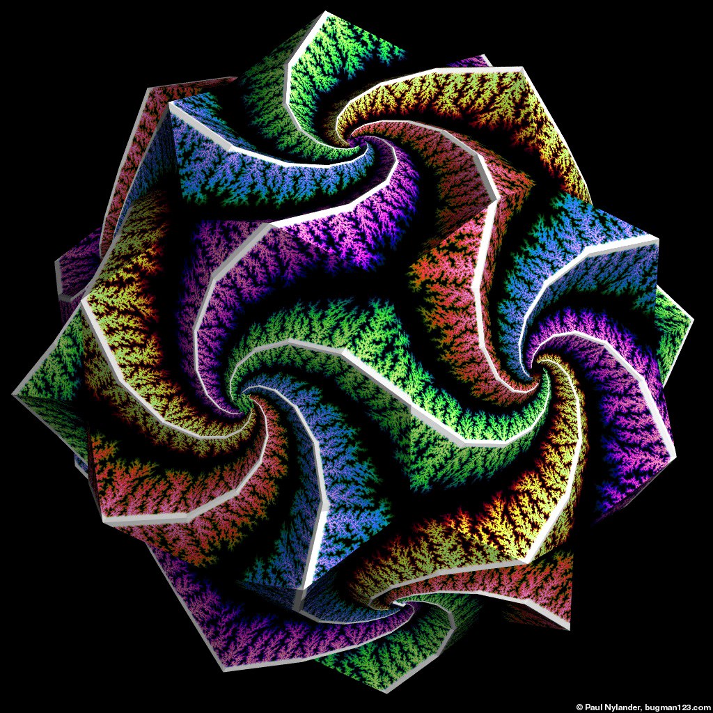
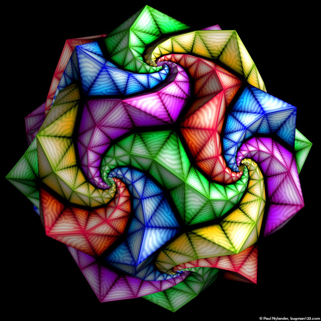

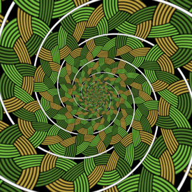
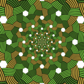
 A spidroball can be formed by applying folded spidrons to the surface of a polyhedron. The concept was originally developed by Daniel Erdely, Amina Buhler, and Marc Pelletier. This example shows a dodeca-spidroball formed by applying spidron tilings with 5 spiral arms to the surface of a dodecahedron. The left image is decorated with Diffusion Limited Aggregation (DLA) fractals, and the right image is decorated with Poisson's Equation and a Reaction-Diffusion pattern. Click here to download some POV-Ray code and here for some AutoLisp code. Here is some Mathematica 8.0 code:
(* runtime: 0.1 second *) Ry[t_] := {{Cos[t], 0, Sin[t]}, {0, 1, 0}, {-Sin[t], 0, Cos[t]}}; Rz[t_] := {{Cos[t], -Sin[t], 0}, {Sin[t], Cos[t], 0}, {0, 0, 1}}; n = 6; t2 = Pi/5; t1 = t2/2; alpha = ArcCos[-Sqrt[5.0]/5]; dz = Sin[t1]^2 Tan[alpha/2]; z = GoldenRatio Tan[alpha/2]/2 + dz; scale = (Cos[t1] - Sqrt[3.0 (1 - Cos[t2])/2])/(2 Cos[t2] - 1); R = scale Rz[ArcCos[Cos[t1] + dz^2 (scale - 1)^2/(2 scale)]]; verts = {}; verts0 = Table[{Cos[i t2], Sin[i t2], (2 Mod[i, 2] - 1) dz}, {i, 0, 9}]; Do[verts = Join[verts, Map[{0, 0, z} + # &, verts0]]; verts0 = Map[R.# &, verts0], {n + 1}]; faces = Flatten[Table[10 i + {{j, Mod[j, 10] + 1, j + 10}, {j + 1, j + 10, Mod[j + 10, 20] + 1}}, {i, 0, n - 1}, {j, 1, 10}], 2]; ToPolys[verts_, faces_] := Map[Polygon[verts[[#]]] &, faces]; Show[Graphics3D[{ToPolys[verts, faces], Table[{ToPolys[Map[Rz[t + t2].Ry[Pi - alpha].# &, verts], faces], ToPolys[Map[Rz[t].Ry[alpha].Rz[t2].# &, verts], faces]}, {t, 2 t2, 2 Pi, 2 t2}], ToPolys[Map[Ry[Pi].# &, verts], faces]}]] |
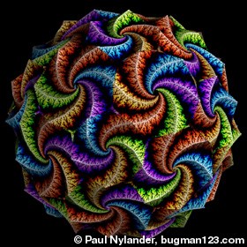 Here is a more complicated spidroball composed of Spidron tilings with 5 and 6 spiral arms covering a truncated icosahedron. I believe it is possible to colorize this spidroball in a more symmetrical way (like the above images), but I haven't taken the time to figure it out.
Links Spidronized Archimedean Solids - higher order Spidroballs, by Walt van Ballegooijen, Marc Pelletierm Amina Buhler-Allen, and Daniel Erdely Spidron Archiball - truncated icosahedron Spidroball, by Walt van Ballegooijen and Marc Pelletier Dodeca-Spidron Ball - by Marc Pelletier and Regina Markus Spidroball - rhombic triacontahedron 3D Spidron Tessellation - fascinating animation, they should manufacture these as toys Spidroball Sculpture - large sculpture Krystyna Burczyk - beautiful origami polyhedrons with no creases Double Spiral - folded out of paper, by David Huffman Whishboneahedron - another interesting design by Florian Sanwald Frabjous - laser-cut wood, by George Hart |
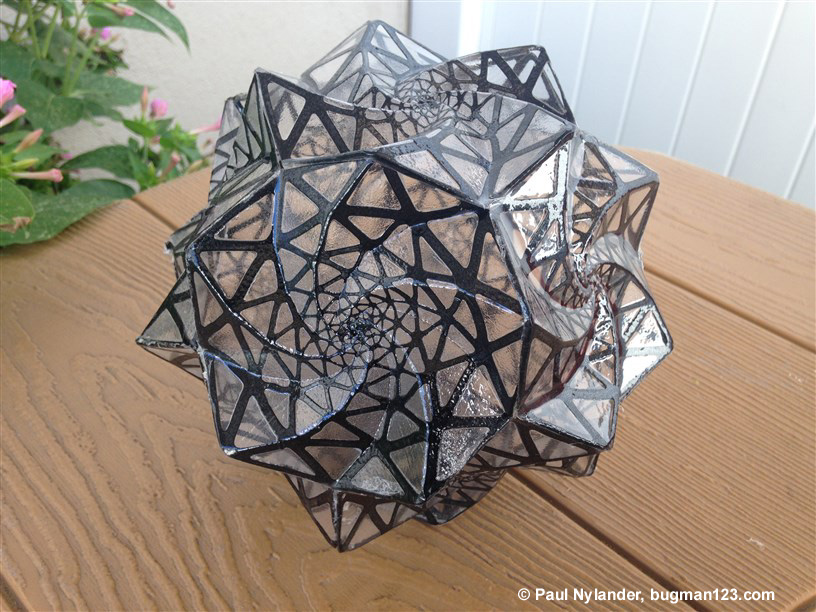
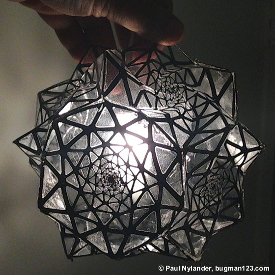
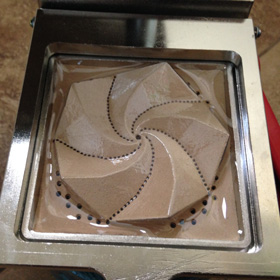
Vacuum Formed Dodeca-Spidroball Lamp - 6/17/17
|
|
Here is a spidroball lamp that I vacuum formed using a cheap dental vacuum forming machine for $80. My goal was to give the illusion of glass mosaic tiles, inspired after Moravian star pendant lamps. It would also be interesting to add slight color tinting and/or frosted surfaces to the windows. One drawback of vacuum forming is that it is highly sensitive to minor variations, resulting in printed patterns that do not always line up correctly with the mold form. Also, vacuum formed parts must be cut out which is time consuming. |
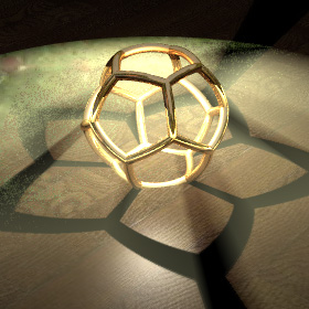
Laser Cut Dodeca-Spidroball Lamps - 7/18/16
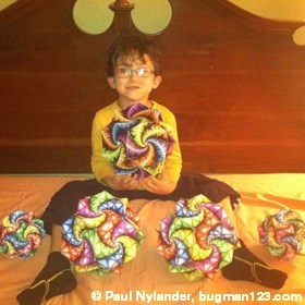 Here are some older spidroball lamps I made using a laser cutter.
 |
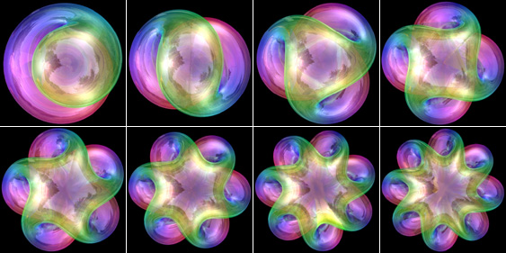
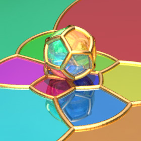
Dodecaplex (120 Cell) - Mathematica 4.2, POV-Ray 3.6.1, 10/21/08
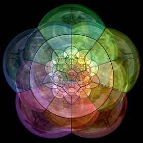
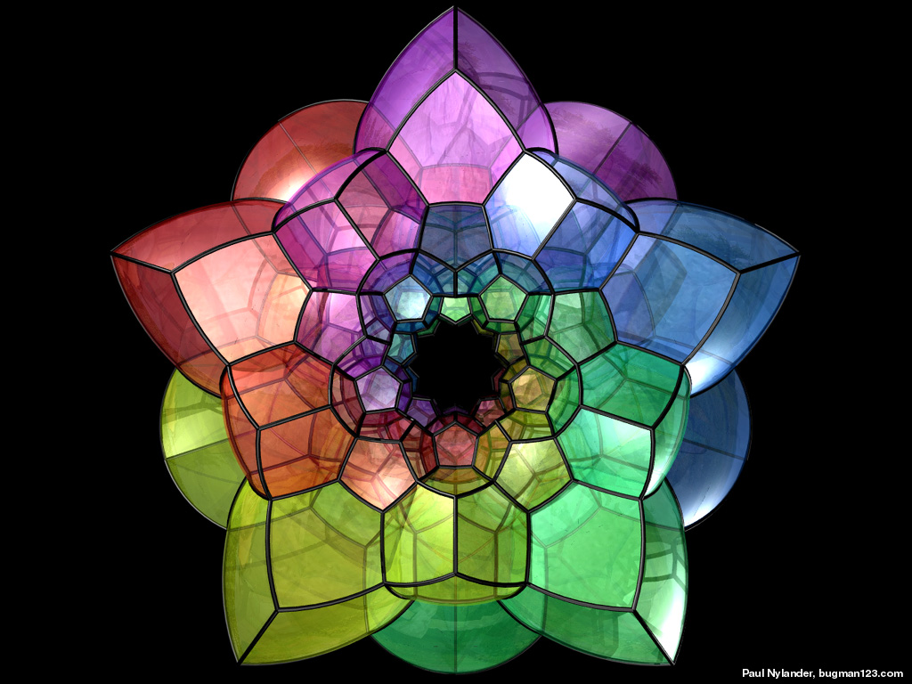

 Polychorons are the 4D version of polyhedrons (in general, for arbitrary dimensions, these are called polytopes). A dodecaplex is a uniform polychoron composed 120 dodecahedral cells. These cells can be divided into 12 rings (Hopf fibrations) of 10 cells each. One way to visualize a polychoron is to apply a 4D to 3D stereographic projection to it. When applied to the dodecaplex, this projection resembles soap bubbles because all intersecting surfaces meet each other at angles of exactly 120°. The left picture shows a stereographic projection of the complete dodecaplex. The right picture shows 6 of the inner rings (each ring is shown in a different color), but only 5 rings are open to direct view because they are wrapped around the 6th ring. I first saw this concept on Matthias Weber's book page. Click here to download some POV-Ray code. You can purchase this as a poster here.
Links Flatland - movie based on Edwin Abbott's novel Jenn 3D - polytope program that uses the Todd-Coxeter algorithm, by Fritz Obermeyer The HyperSphere, from an Artistic point of View - explanation by Rebecca Frankel 120 Cell Soap Bubbles - by John Sullivan Magic 120 Cell - YouTube video demonstrating how to solve this complicated variation of the Rubik's Cube, by Noel Chalmers Regular Polytopes - Mathematica notebook by Russell Towle POV-Ray include files - by Russell Towle Magic 120 Cell - OpenGL program by Roice Nelson, et al. |
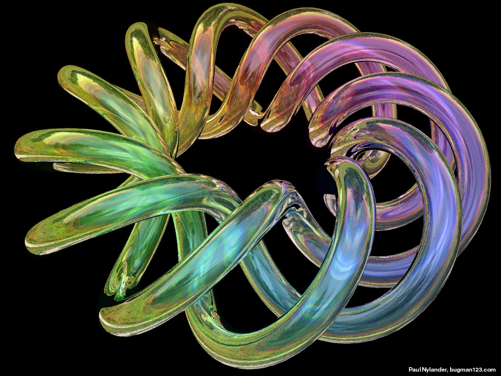
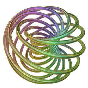
Hopf Fibration - Mathematica 4.2, POV-Ray 3.6.1, 8/12/08


 The Hopf map is a special transformation invented by Heinz Hopf that maps to each point on the ordinary 3D sphere from a unique circle of points on the 4D sphere. Taken together, these circles form a fiber bundle called a Hopf Fibration. If you apply a 4D to 3D stereographic projection to the Hopf Fibration, you get a beautiful 3D torus called a Clifford Torus composed of interlinked Villarceau circles. By applying 4D rotations to the Hopf Fibration, you can transform the Clifford Torus into a Dupin cyclide or you can turn it inside-out. There is a single point of rotation in 2D, there are 3 axes of rotation in 3D (x, y, z), and there are 6 planes of rotation in 4D (xy, xz, xw, yz, yw, zw). Click here to download some POV-Ray code. Here is some Mathematica code:
(* runtime: 7 seconds *) HopfInverse[theta_, phi_, psi_] := {Cos[phi/2] Cos[psi], Cos[phi/2]Sin[psi], Cos[theta + psi]Sin[phi/2], Sin[theta + psi]Sin[phi/2]}; Ryw[theta_] := {{1, 0, 0, 0}, {0, Cos[theta], 0, Sin[theta]}, {0, 0, 1, 0}, {0, -Sin[theta], 0, Cos[theta]}}; StereographicProjection[{x_, y_, z_, w_}] := {x, y, z}/(1 - w); Table[Show[Graphics3D[Table[{Hue[(4 phi/Pi - 1)/3],Table[Line[Table[StereographicProjection[Ryw[alpha].HopfInverse[theta, phi, psi]], {psi, 0.0, 2Pi, Pi/18}]], {theta, 0.0, 2 Pi,Pi/9}]}, {phi, Pi/4, 3Pi/4, Pi/4}], PlotRange -> 3{{-1, 1}, {-1, 1}, {-1, 1}}]], {alpha, 0, Pi, Pi/18}]; |
 Links
LinksDimensions - interesting video animated by Jos Leys, see their fibration explanation and video Hopf Fibration, Clifford Torus - 3D prints, by Henry Segerman Torofluxus - cool toy invented by Jochen Valett, you can buy one here The Flat Torus in 3-Sphere - by Thomas Banchoff, explanation1, explanation2, animations Stereographic Projection - by Davide Cervone Visualization of the Hopf Bundle - Mathematica notebook by Srdjan Vukmirovic Hyperspheres - If a 1-sphere is a circle, and a 2-sphere is a regular sphere, then what is a 3-sphere? How about a 4.5-sphere? Did you know there is a formula to find the “volume” for any n-sphere? |
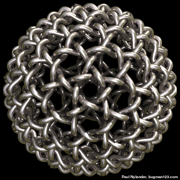
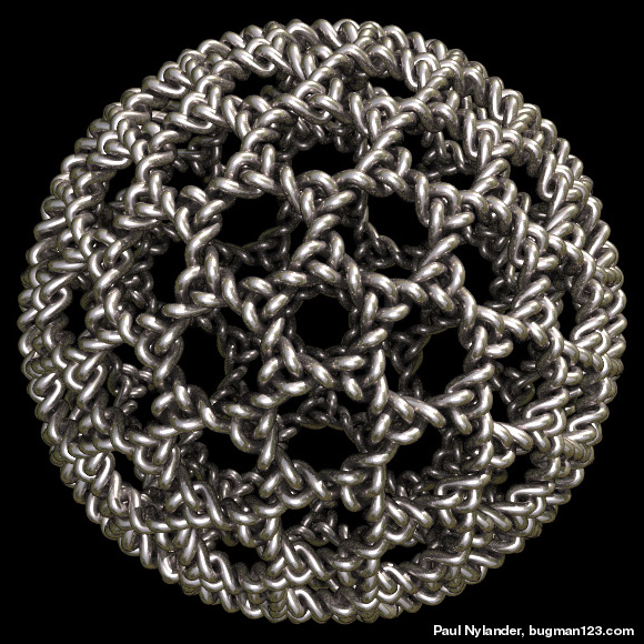
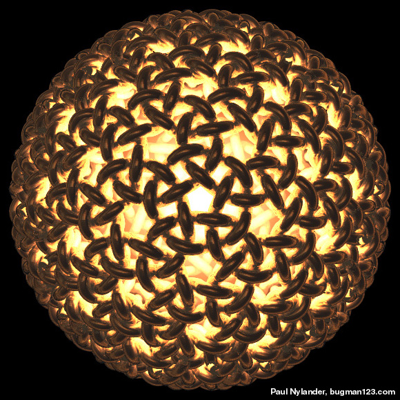
Geodesic Sphere Knots - Mathematica 4.2, POV-Ray 3.6.1, 2/15/11
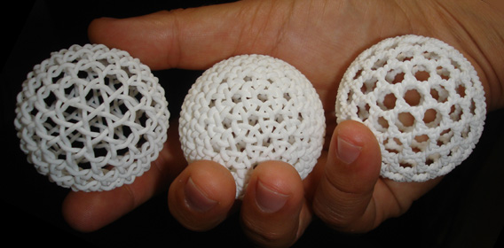
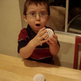 There are many ways to cover surfaces with a network of knots. You can purchase these 2 inch or 1 inch geodesic sphere knots here. They are not recommended for children's toys, but they are somewhat durable and bouncy (my 2 year old son approved of them). You can insert small LEDs and hang them as pendant lamps, or use them as Christmas tree ornaments, or hang them from your rear view mirror.
Links Geo Weave, Geodesic Weave, Worm Weave, Takraw Ball Toy (Dick Esterle's Nobbly Wobbly) - beautiful renderings by Taff Goch, see also this analysis International Guild of Knot Tyers - we recently saw this group at the Tall Ships Festival, be sure to see the animals and Turk's Head globes Celtic knotwork tutorial - by Christian Mercat Bending a Soccer Ball - animations by Michael Trott KnotsBag - software by Hypatiasoft Knots3D - free Celtic knot program by Steve Abbott, see also KnotsBag by Geraud Bousquet The KnotPlot Site - interesting knots by Robert Scharein, some of my favorites are his Brunnian Links, Ashley Knot #2445 and #2462, bbframe-bain6b, and 13jun03d2 3D Printing Links Homemade SLA printer - by Junior Veloso 3D Printed Candy - trefoils, dodecahedrons, moebius strips, created with the CandyFab 6000 D-Shape - large scale 3D printing for buildings |


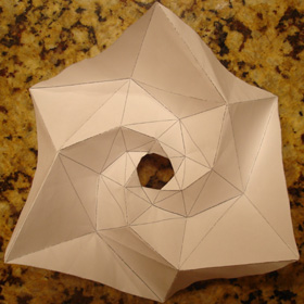
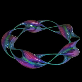
Knotted Surface - AutoCAD 2000, POV-Ray 3.6.1, 4/24/07
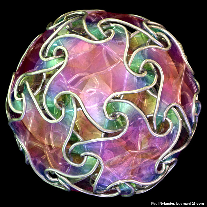

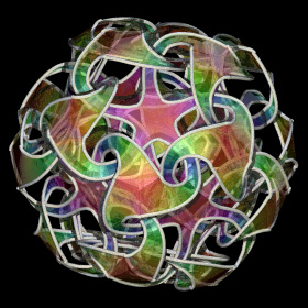
 This began as an attempt to animate a similar-looking structure to Bathsheba Grossman’s beautiful Quin Pendant Lamp. To create this image, first I sketched the basic curves for one arm in AutoCAD and then I assembled and rendered it in POV-Ray. Depending on your point of view, this knotted surface can be seen as a dodecahedron with a hole over each edge, or an icosahedron with a hole over each vertex, or an icosahedron with a hole over each edge, or a rhombic triacontahedron with a hole over each face. The left animation shows a homotopy that continuously maps the structure into a sphere with 30 holes. The boundary of each hole loops over itself twice and links with 6 others. This image was featured on the cover of McGraw-Hill's 2012 & 2013 Algebra 2 textbooks. Here is some Mathematica code:
(* runtime: 0.1 second *) << Graphics`Shapes` ; alpha = ArcCos[-Sqrt[5]/5]; surface = {{{0.11, 0.35, 1}, {0.16, 0.33, 1}, {0.23, 0.35, 0.99}, {0.3, 0.38, 0.96}, {0.35, 0.43, 0.9}, {0.29, 0.42, 0.8}, {0.22, 0.37,0.7}, {0.14, 0.34, 0.62}, {0.078, 0.296, 0.585}}, {{0, 0, 1}, {0.13, 0.09, 1}, {0.29, 0.22, 0.99}, {0.4, 0.33, 0.95}, {0.41, 0.45, 0.88}, {0.31, 0.47, 0.77}, {0.2, 0.43, 0.65}, {0.08, 0.4, 0.56}, {-0.019, 0.398, 0.526}}, {{0.36, 0, 1}, {0.39, 0.11, 1}, {0.45, 0.23,0.99}, {0.49, 0.35, 0.95}, {0.47, 0.45, 0.86}, {0.36, 0.52, 0.73}, {0.22, 0.5, 0.59}, {0.13, 0.48, 0.48}, {0.07, 0.489, 0.437}}}; arm = Map[Polygon[Flatten[#, 1][[{1, 2, 4, 3}]]] &, Partition[surface, {2, 2}, 1], {2}]; face = Table[RotateShape[Graphics3D[arm], 0, 0, psi][[1]], {psi, 0, 1.6Pi, 0.4Pi}]; Show[Graphics3D[{face, RotateShape[face, 0, Pi, 0], Table[{RotateShape[face, 0, Pi - alpha, psi + Pi/5], RotateShape[face, Pi/5, alpha, psi]}, {psi, 0, 1.6Pi, 0.4Pi}]}]] |
 Links
LinksQuin Pendant Lamp - a very beautiful lamp by Bathsheba Grossman Starfish Bling Ball - gorgeous jeweled version, by Florian Sanwald Nexus - another one of my favorites by Bathsheba Grossman Linking Stars - also inspired after Bathsheba Grossman's Quin Lamp, created by Jonathan Johanson using TopMod3d, see also his rotatable model Icosahedron VI - similar sculpture by Vladimir Bulatov, see also his pendant Linking Stars - video tutorial how to create these using TopMod3d, by sjo.Johanson Irregular Detail - an interesting design by Florian Sanwald, hard to figure out Pocket Art - impressive wood carvings of polyhedral knots, by Bjarne Jespersen, see also his explanation Life Support - interesting 3D printed model with dodecahedral symmetry, by Stijn van der Linden TopMod3d - free topological mesh modeling software Metal Printed Quintrino - by Bathsheba Grossman Mysterious Star - interesting shape, by Mehrdad Garousi IQ-light (Interlocking Quadrilaterals) - by Holger Strřm Sarah Turner - artist creates lamps from waste plastic drink bottles Knobbyball - beautiful truncated icosahedron design, by Robert Drummond |
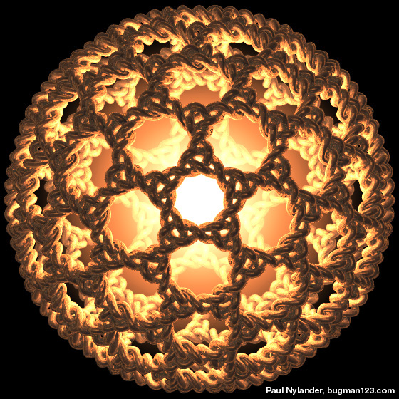
Knotted Geodesic Sphere Surface - Mathematica 4.2, POV-Ray 3.6.1, 3/3/11
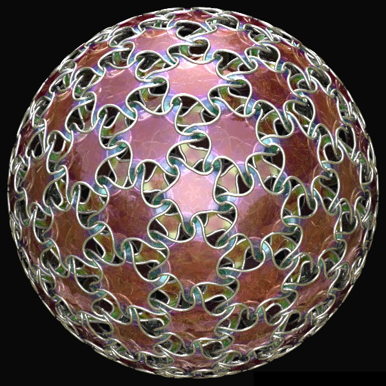
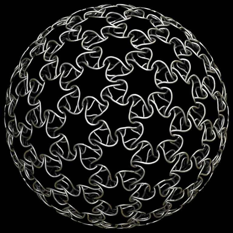
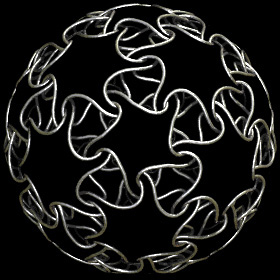 The pattern on this knotted surface was inspired after Bathsheba Grossman’s beautiful Quin Pendant Lamp.
Links Starfishberry - a similar concept by Florian Sanwald, here is another variation by Jonathan Johanson |
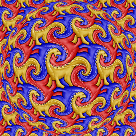
“Rep-Tiles” Dinosaur Tessellation - AutoCAD 2000, AutoLisp, Adobe Photoshop 5.0, 12/9/02
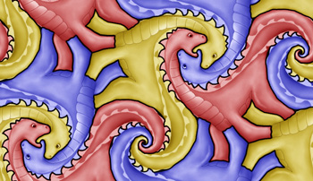
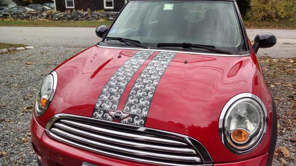 A tessellation is a regular tiling of figures without any gaps or overlapping. If you have access to AutoCAD, you can use this AutoLisp routine to help you design your own tessellations. You can purchase pattern as a tie or as a printed fabric. The right photo shows this tessellation on a car.
Tessellation Links Penrose Tiling Java Applet - by Craig Kaplan Maurits Cornelis Esher (M.C. Escher) - famous artist who used tessellations in his artwork Tessellation Java Applet - create your own tessellations I Love Dragons - a nice looking reproduction of this tessellation by a student at Lizzie M. Burges Alternative School |
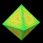
Polyhedrons with Reaction-Diffusion Patterns - new version: C#, POV-Ray 3.6.1, 12/1/11; old version: C++, Mathematica 4.2, 5/24/07
(* runtime: 7 minutes *) n = 80; w = 0.35; SeedRandom[0]; image = Table[Random[Integer, {0, 1}], {n}, {n}]; Do[image = Table[ID = AD = 0; Do[If[image[[Mod[i + di - 1, n] + 1, Mod[j + dj - 1, n] + 1]] == 1, r = Sqrt[di^2 + dj^2]; If[3 <= r <= 6, ID++]; If[r <= 3, AD++]], {di, -6, 6}, {dj, -6, 6}]; a = AD - w ID; Which[a > 0, 1, a < 0, 0, True, image[[i, j]]], {i, 1, n}, {j, 1, n}]; ListDensityPlot[image, Mesh -> False, Frame -> False], {10}]; Links Xmorphia - detailed simulation demonstrating varying parameters, by Robert Munafo (originally by Roy Williams) Gray-Scott Reaction-Diffusion - Java applet by Jonathan Lidbeck Heated metal alloy simulation - Java applet by Thomas Wanner Activator-Inhibitor - Wolfram Demonstrations Project Cahn-Hilliard equation |
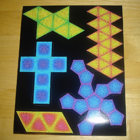
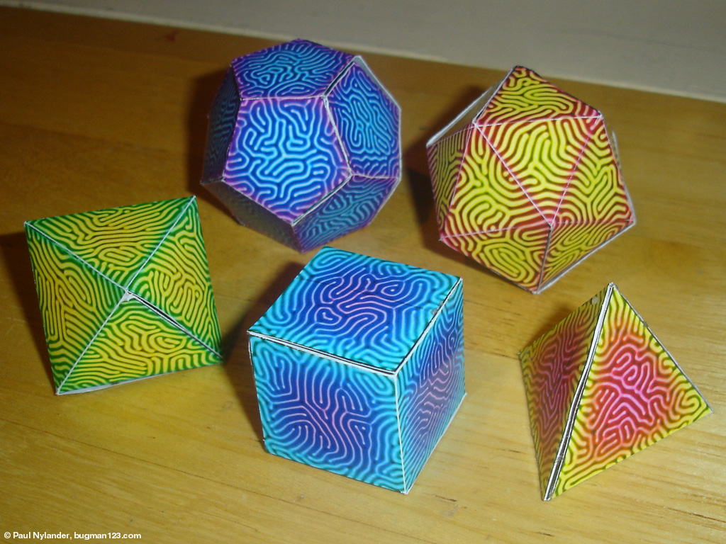
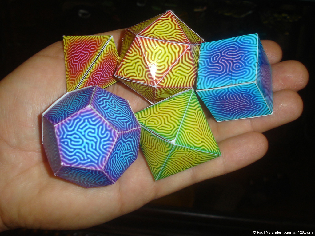
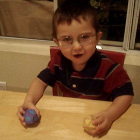 Here are some platonic solids that I made for my 2 year old son. They were cut and folded from this template of printed photos. Most babies only get to play with 2D shapes, but if these could be baby-proofed, I think they would be a fun way to introduce 3D geometry to kids at an early age. Even most adults are not familiar with many of these solids.
 |
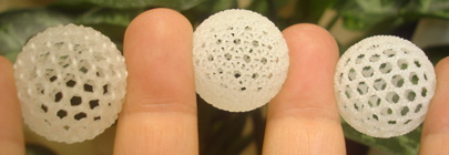
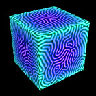
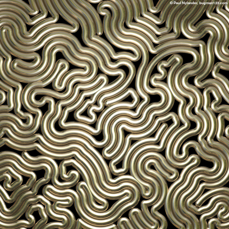
Spherical Cube with Reaction-Diffusion Pattern - C#, POV-Ray 3.6.1, 11/25/11
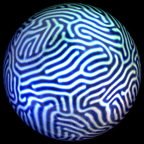
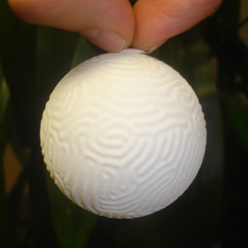
 When we tried to map a Reaction-Diffusion pattern to a sphere using spherical coordinates, the integration became unstable at the poles. As an alternate approach, Daniel Walsh proposed a clever formula for mapping the pattern onto a cube that can be projected undistorted onto the sphere. Here is my rendition of a sphere using this approach. You can purchase 3D prints of this here. The 2 inch sphere costs about $10, and the 1 inch sphere costs about $8.
Links Reaction Seed Lamp 1, Seed Lamp 2, Spiral Lamp, Reaction Vase - beautiful 3D printed models, by Nervous Systems Neri Oxman - MIT media arts professor explores possibilities of 3D printing ReactionDiffusionSphere01, ReactionDiffusionSphere03 - by Michael Spaw |
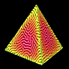
Knotted Surface with Reaction-Diffusion Pattern - C#, POV-Ray 3.6.1, 12/9/11
 Reaction-Diffusion patterns can also be applied to arbitrary meshes. However, the pattern can become distorted if the mesh faces have corner angles that are too sharp, as you can see here. Maybe I'll try to make a better looking version of this if I have time.
 |
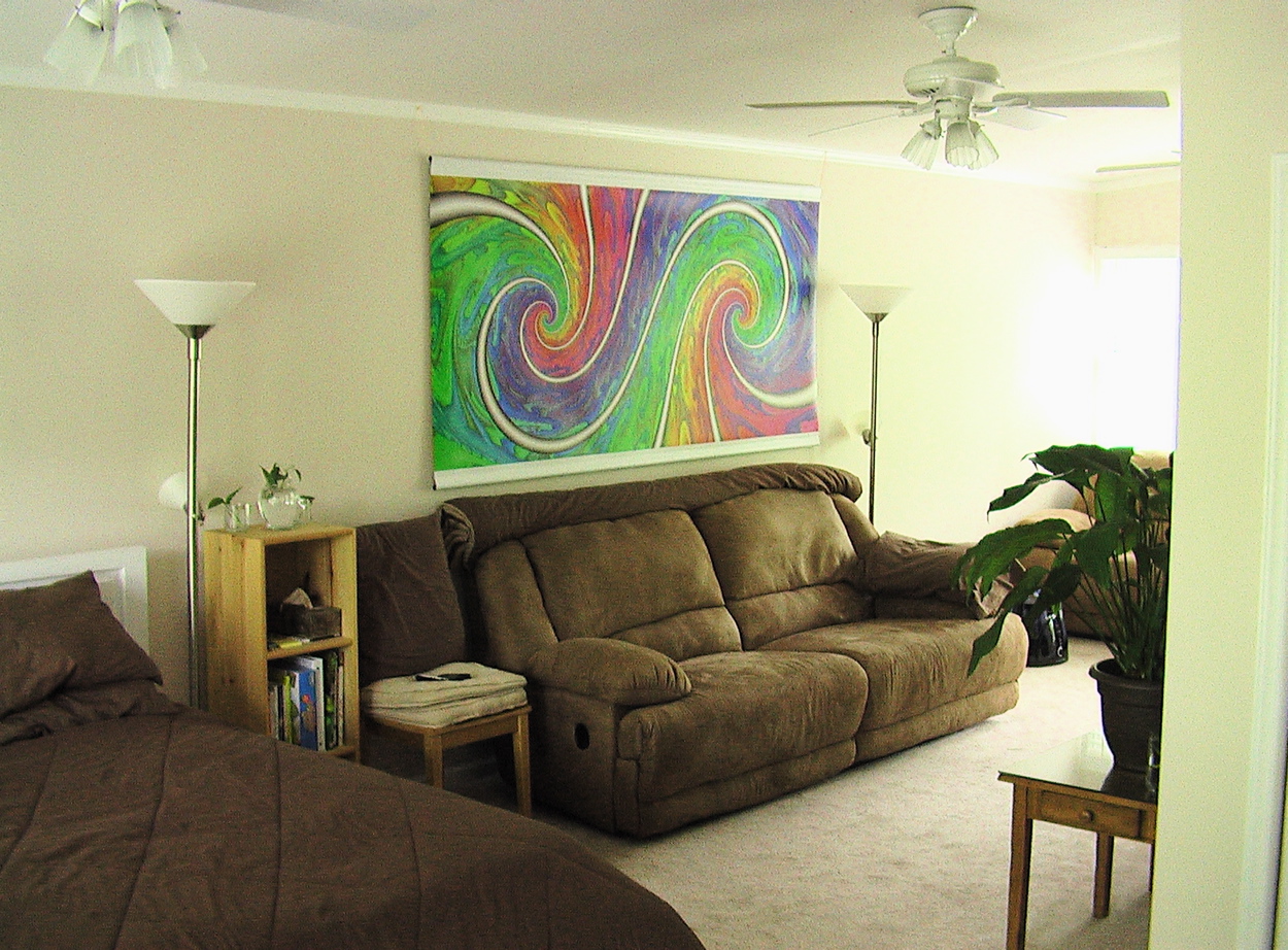
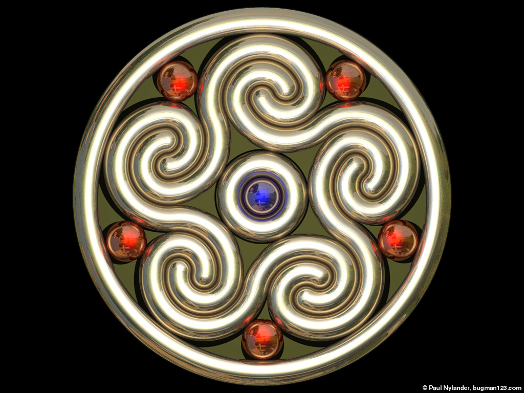
Stereographic Projection of a Loxodrome - new version: C++, POV-Ray 3.6.1, 10/1/08; old version: Mathematica 4.2, 7/18/05

 You can purchase this as a poster here and here. Click here to download a Mathematica notebook. Here is some Mathematica code:
(* runtime: 3 seconds *) << Graphics`Shapes`; a = 0.25; Rx[phi_] := {{1, 0, 0}, {0, Cos[phi], -Sin[phi]}, {0, Sin[phi], Cos[phi]}}; Do[loxodrome = Table[Rx[phi].{Sin[t], -a t, -Cos[t]}/Sqrt[1 + (a t)^2], {t, -100, 100, 0.1}]; projection = Map[Module[{r = 2/(1 - #[[3]])}, {r #[[1]],r #[[2]], -1}] &, loxodrome]; Show[Graphics3D[{EdgeForm[], Sphere[0.99, 37, 19], Polygon[{{4, 4, -1}, {-4, 4, -1}, {-4, -4, -1}, {4, -4, -1}}],Line[loxodrome], Line[projection]},PlotRange -> {{-4, 4}, {-4, 4}, {-1, 1}}]], {phi, 0, Pi -Pi/12, Pi/12}] Links Triply Orthogonal System and Loxodrome Surface - amazing 3D versions of this concept, by Daniel Piker |
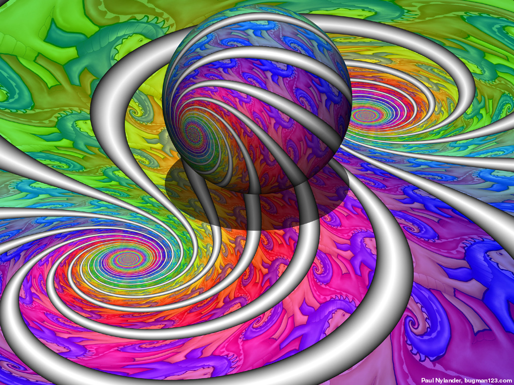
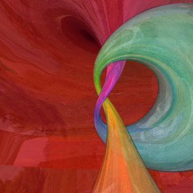
Homography of a Logarithmic Spiral - new version: C++, 10/1/08; old version: Mathematica 4.2, 7/18/05

 Another kind of double spiral can be made by applying a special homography to a single logarithmic spiral:
(* runtime: 0.05 second *) Show[Graphics[Table[Line[Table[z = Exp[r + (2 r + theta)I]; z = (1 + z)/(1 - z); {Re[z], Im[z]}, {r, -10, 10, 0.1}]], {theta, -Pi, Pi, Pi/3}], PlotRange -> {{-2, 2}, {-2, 2}}, AspectRatio -> Automatic]] Here is some Mathematica code that uses the inverse method: (* runtime: 17 seconds *) Show[Graphics[RasterArray[Table[r1 = (x - 1)^2 + y^2; r2 = (x + 1)^2 + y^2; Hue[(Sign[y]ArcCos[(x^2 + y^2 - 1)/Sqrt[r1 r2]] -Log[r1/r2])/(2Pi)], {x, -2, 2, 4/274}, {y, -2, 2, 4/274}]], AspectRatio -> 1]] and here is some POV-Ray code: // runtime: 2 seconds camera{orthographic location <0,0,-2> look_at 0 angle 90} #declare r1=function(x,y) {(x-1)*(x-1)+y*y}; #declare r2=function(x,y) {(x+1)*(x+1)+y*y}; #declare f=function{(y/abs(y)*acos((x*x+y*y-1)/sqrt(r1(x,y)*r2(x,y)))-ln(r1(x,y)/r2(x,y)))/(2*pi)}; plane{z,0 pigment{function{f(x,y,0)}} finish{ambient 1}} The photo on the right shows a giant 91 inch poster of this image. Please email me if you are interested in purchasing a giant poster of any of my art creations. You can also purchase smaller posters here. Links other double spiral formulas - Cornu spiral (clothoid), tanh spiral Whirlpools - famous double spiral tessellation by M.C. Escher Double Spiral - folded out of paper, by David Huffman |
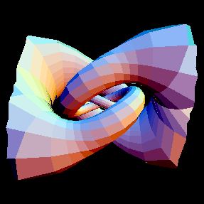
Boy’s Surface (Bryant-Kusner Parametrization) - new version: POV-Ray 3.6.1, 6/20/06
old version: Mathematica 4.2, MathGL3d, POV-Ray 3.6.1, 5/24/05
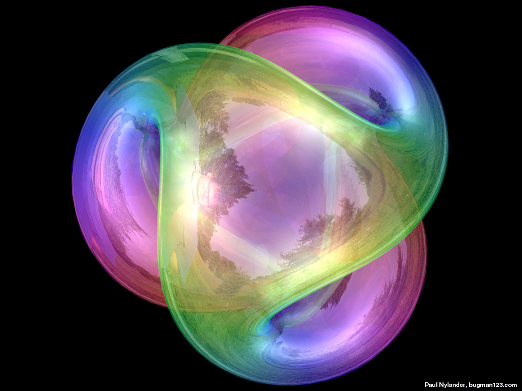

 This Boy’s Surface is a one-sided surface that was first parametrized correctly by Bernard Morin. The left animation looks like it’s turning inside-out (although technically that’s impossible because it only has one side). Robert Bryant told me that the parameters (p,q) = (0,1) give this Willmore immersion of RP2 a trilateral symmetry and the parameters (p,q) = (1,0) should give bilateral symmetry. This image was printed on the cover of McGraw-Hill's 2012 Pre-Algebra textbook. Click here to download some POV-Ray code for this image and here for some AutoLisp code. Here is some Mathematica code:
(* runtime: 1 second *) ParametricPlot3D[Module[{z = r E^(I theta), a, m}, a = z^6 + Sqrt[5]z^3 - 1; m = {Im[z(z^4 - 1)/a], Re[z(z^4 + 1)/a], Im[(2/3) (z^6 + 1)/a] + 0.5}; Append[m/(m.m), SurfaceColor[Hue[r]]]], {r, 0, 1}, {theta, -Pi, Pi}, PlotPoints -> {20, 72}, ViewPoint -> {0, 0, 1}] POV-Ray also has an internal function for a different parametrization: // runtime: 50 seconds camera{location -1.5*z look_at 0} light_source{-z,1} #declare f=function{internal(8)} isosurface{function{-f(x,y,z,1e-4,1)} pigment{rgb 1}} Links Rotatable 3D Boy’s Surface Steiner Surfaces - POV-Ray animations by Adam Coffman |
 Another way to obtain other symmetries is to apply a mapping transformation. The n = 1 case is a Klein bottle.
Klein Bottle and Möebius Strip Links Möebius Strip - a simple one-sided surface, see these twisting and 5 fold animated Möebius strips by Jos Leys Twin Rail Mobius Pendant - metal Mobius with ball bearings, by Paul King Hand-Blown Glass Klein Bottles - by Cliff Stoll Nested Klein Bottles - by Alan Bennett Möebius strip to Klein bottle transformation - Mathematica code by Ari Lehtonen Trefoil Knot Minimal Surface - by Nat Friedman |
Spidron - folded paper, POV-Ray 3.6.1, 7/28/10
 Spidrons were invented by Daniel Erdely in 1979 as a homework assignment for Erno Rubik, inventor of the Rubik's Cube. Spidrons can folded into expandable 3D shapes and can be applied to polyhedrons and tessellations. The original spidron can form a tiling with 3 spiral arms. Click here to download some POV-Ray code. Here is some Mathematica code:
(* runtime: 0.01 second *) n = 5; elems = Flatten[Table[6i + {{j, Mod[j, 6] + 1, j + 6}, {j + 1, j + 6, Mod[j + 6, 12] + 1}}, {i, 0, n - 1}, {j, 1, 6}], 2]; Do[r = Sqrt[1 - 4dz^2]; dtheta = ArcCos[(1 + 2 Sqrt[3] + 1/(4dz^2 - 1))/4];R = {{Cos[dtheta], -Sin[dtheta], 0}, {Sin[dtheta], Cos[dtheta], 0}, {0, 0, 1}}/Sqrt[3]; nodes0 = nodes = Table[{r Cos[i Pi/3], r Sin[i Pi/3], (2Mod[i, 2] - 1) dz}, {i, 0, 5}]; Do[nodes0 = Map[R.# &, nodes0];nodes = Join[nodes, nodes0], {n}]; Show[Graphics3D[Map[Polygon[nodes[[#]]] &, elems], PlotRange -> {{-1, 1}, {-1, 1}, {-1, 1}}]], {dz, 0.0, 1/3, 0.05}] Spidron Links Spidron Relief - folding tessellation animation Spidron Exhibition Tile Magic - by Akira Nishihara |
7 Arm Sphidron - POV-Ray 3.6.1, 7/21/10
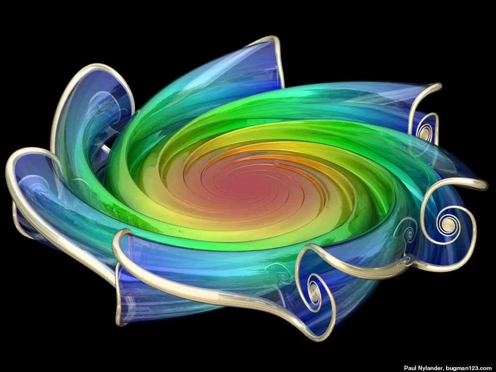
 Another one of Daniel Erdely's inventions are sphidrons. Sphidrons are similar to spidrons except they are smooth. I am not exactly sure what defines this surface, but this image uses a spiral wave based on a double spiral. Now, here is the big question: is it possible to "roll" a single piece of paper into a shape that looks something like this, without stretching the paper?
Links 6 Arm Sphidron - YouTube animation, here is another animation Paper Sphidrons - by Daniel Erdely Double Spiral - folded out of paper, by David Huffman |
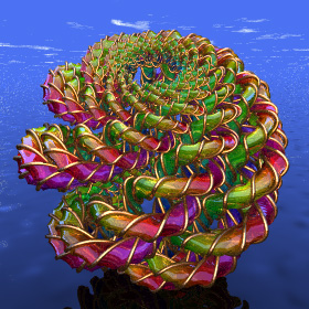
"Math Rose" - new version: POV-Ray 3.6.1, 6/21/06
old version: Mathematica 4.2, MathGL3d, 3/5/04
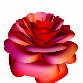

 This rose is actually a plot of a single, continuous, parametric math equation. I got this idea while trying to create a visualization of a spiraling spin-lattice relaxation for a physics experiment involving a Nuclear Magnetic Resonance (NMR) spectrometer. You can purchase a 3D printed version of this rose here. Click here to see a larger animation. Click here to see a rotatable 3D version. Click here to download some POV-Ray code for this image and here for some AutoLisp code. See also my Passion Flower. Here is some Mathematica code:
(* runtime: 16 seconds *) Rose[x_, theta_] := Module[{phi = (Pi/2)Exp[-theta/(8 Pi)], X = 1 - (1/2)((5/4)(1 - Mod[3.6 theta, 2 Pi]/Pi)^2 - 1/4)^2}, y = 1.95653 x^2 (1.27689 x - 1)^2 Sin[phi]; r = X(x Sin[phi] + y Cos[phi]); {r Sin[theta], r Cos[theta], X(x Cos[phi] - y Sin[phi]), EdgeForm[]}]; ParametricPlot3D[Rose[x, theta], {x, 0, 1}, {theta, -2 Pi, 15 Pi}, PlotPoints -> {25, 576}, LightSources -> {{{0, 0, 1}, RGBColor[1, 0, 0]}}, Compiled -> False] Links This rose is featured in Ramiro Perez's Incendia software (see his Rose Curve and Rose Gasket) A Rose for Valentine's Day - adaptation for Wolfram Demonstration Project, by Jeff Bryant A Rose for Aexion - another rendering of this rose by parrotdolphin |
Seifert Surfaces - POV-Ray 3.6.1, 9/24/12
 A Seifert surface is a surface whose boundary is a knot or a link. Some Seifert surfaces can also be minimal surfaces. The following Mathematica code was adapted from Jos Leys' PovRay code for a Seifert trefoil:
(* runtime: 1 second *) << Graphics`Master`; StereographicProjection[{x_, y_, z_, w_}] := {x, y, z}/(1 - w); f[phi_, v_] := Module[{g4 = phi + I vsign Log[1 - v]}, g2 = ((1 + Sin[g4])/(2Sqrt[2]))^(1/3); g3 = Sqrt[(Sin[g4] - 1)/2]; f[k_] := k^3Abs[g3]^2 + k^2 Abs[g2]^2 - 1; k0 = 0.0; k = 1.0; While[Abs[k - k0] > 1.0*^-6, k0 = k;k = k0 - f[k0]/f'[k0]];g2 *= k Exp[I theta]; g3 *= sign k^1.5; StereographicProjection[{Im[g2], Re[g2], Im[g3], Re[g3]}]]; DisplayTogether[Table[ParametricPlot3D[f[phi, v], {phi, -Pi/2, Pi/2}, {v, 0, 1}, PlotPoints -> {20, 10},DisplayFunction -> Identity], {vsign, -1, 1, 2}, {sign, -1, 1, 2}, {theta, 0, 4 Pi/3, 2 Pi/3}], ViewPoint -> {0, 0, 1}] Links SeifertView - free program for creating knotted surfaces, by Jarke van Wijk and Arjeh Cohen Lorenz and Modular Flows - by Jos Leys, and Etienne Ghys Borromean Rings - Seifert surface, by Bathsheba Grossman |
Torus with Knotted Hole - POV-Ray 3.6.1, 7/31/12
 Here is a 4D rotation of a trefoil transforming into a torus with a knotted hole. In general, you can continuously turn any 3D object "inside-out" by applying an inverse stereographic projection that maps the 3D object onto the surface of a 4D hypersphere, then rotating it in 4D space, and finally applying a forward stereographic projection to return it back to 3D space.
(* runtime: 11 seconds *) StereographicProjection[{x_, y_, z_, w_}] := {x, y, z}/(1 - w); InverseStereographicProjection[p_] := Module[{r2 = Norm[p]}, Append[2 p, r2 - 1]/(r2 + 1)]; Ryw[theta_] := {{1, 0, 0, 0}, {0, Cos[theta], 0, -Sin[theta]}, {0, 0, 1, 0}, {0, Sin[theta], 0, Cos[theta]}}; f[t_] := {(2 + Cos[2 t]) Cos[3 t], (2 + Cos[2 t]) Sin[3 t], Sin[4 t]}/4; rtube = 1.0/6; TubePlot[t_, theta_] := Module[{df = f'[t], ddf = f''[t], x, y, z}, z = Normalize[df]; x = Normalize[ddf (df.df) - df (df.ddf)]; y = Cross[x, z]; f[t] + rtube (x Cos[theta] + y Sin[theta])]; ParametricPlot3D[StereographicProjection[Ryw[Pi/2].InverseStereographicProjection[TubePlot[t, theta]]], {t, 0, 2 Pi}, {theta, 0, 2 Pi}, PlotPoints -> {72, 18}, ViewPoint -> {0, -1, 0}] Links Knot Complement - 4D rotation of trefoil transforming into torus with knotted hole, by Daniel Piker Figure 8 Knot Trumpet - 3D print, by Henry Segerman |
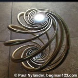
Dodecahedral Loxodrome - Mathematica 4.2, POV-Ray, 10/28/11
 Here is another similar concept to my loxodrome sconce, but with more spirals on it.
 |
“Free Spirit Tessellation” - AutoCAD 2000, AutoLisp, Adobe Photoshop 5.0, 5/12/03
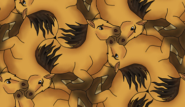 I modeled this tessellation after “Spirit” from Disney’s “Spirit - Stallion of Cimarron” movie. I had to overlap the horse’s hind legs because there was not enough room. Still, I think the rest of it fits together remarkably well.
 |
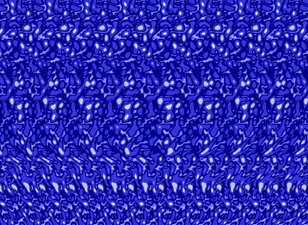
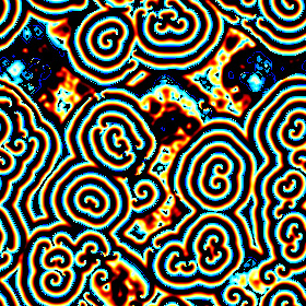
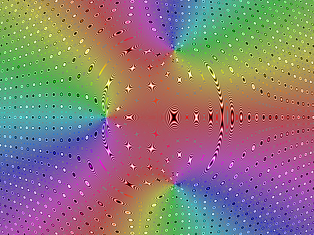
Maelström Autostereogram - Mathematica 4.2, SISgen 1.58, 10/1/04
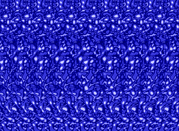
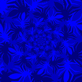
 This 3D vortex image is hidden in the above picture. To see it, relax your eyes and focus behind the screen. This autostereogram was generated with William Steer’s free autostereogram generating program SISgen. Click here to see an animated version of this picture. I also have a Mathematica-only version of this picture, but it is not as accurate. See also Pascal Massimino’s “Maelstrom” autostereogram.
(* Create Depth Map, runtime: 1 minute *) r := Sqrt[x^2 + y^2]; z := 0.03Sin[7(2r - ArcTan[x, y])] - 0.1/r - 0.3; phi = Pi/6; ymax = 1.0/Cos[phi]; j1 = 615; i1 = 450; depth = Table[0, {i1}, {j1}]; Do[flag = False; Do[i0 = ip; ip = Round[(i1 - 1 + (j1 - 1) (y Cos[phi] + z Sin[phi]))/2 + 0.2i1] + 1; z2 = z1; z1 = -y Sin[phi] + z Cos[phi]; If[flag, sign = If[i0 < ip, 1, -1]; j = Round[(j1 - 1)(x + 1)/2] + 1; Do[If[0 < i <= i1, depth[[i, j]] = ((i - i0)z1 + (ip - i)z2)/(ip - i0)], {i, i0 + sign, ip, sign}]]; flag = True, {y, ymax, -ymax, -2.0ymax/i1}], {x, -1, 1, 2.0/j1}]; ListDensityPlot[depth, Mesh -> False, Frame -> False, ImageSize -> {j1, i1}, AspectRatio -> Automatic] (* Create Shift Pattern, runtime: 10 seconds *) i2 = 450; j2 = 90; SeedRandom[0]; pattern = Map[Hue, -50Abs[InverseFourier[Fourier[Table[Random[], {i2}, {j2}]]Table[Exp[-((j/j2 - 0.5)^2 + (i/i2 - 0.5)^2)/0.025^2], {i, 1, i2}, {j, 1, j2}]]], {2}]; Show[Graphics[RasterArray[pattern],ImageSize -> {j2, i2}, AspectRatio -> Automatic]] (* Generate Autostereogram, Note: this code is not very accurate, you are better off using SISgen, runtime: 14 seconds *) f[z_] := 2(14 - 8.7z)/(28 - 8.7z); g[sign_] := Module[{x=0}, Table[x += sign/f[depth[[i, j]]]; pattern[[Mod[i - 1, i2] + 1, Mod[Round[x] - 1, j2] + 1]], {j, Floor[j1/2], If[sign != 1, 1, j1], sign}]]; Show[Graphics[RasterArray[Table[Join[Reverse[g[-1]], g[1]], {i, 1, i1}]], ImageSize -> {j1, i1}, AspectRatio -> Automatic]] Link: Animated Shark Autostereogram - by Fred Hsu |
Tetration - Mathematica, 10/8/12
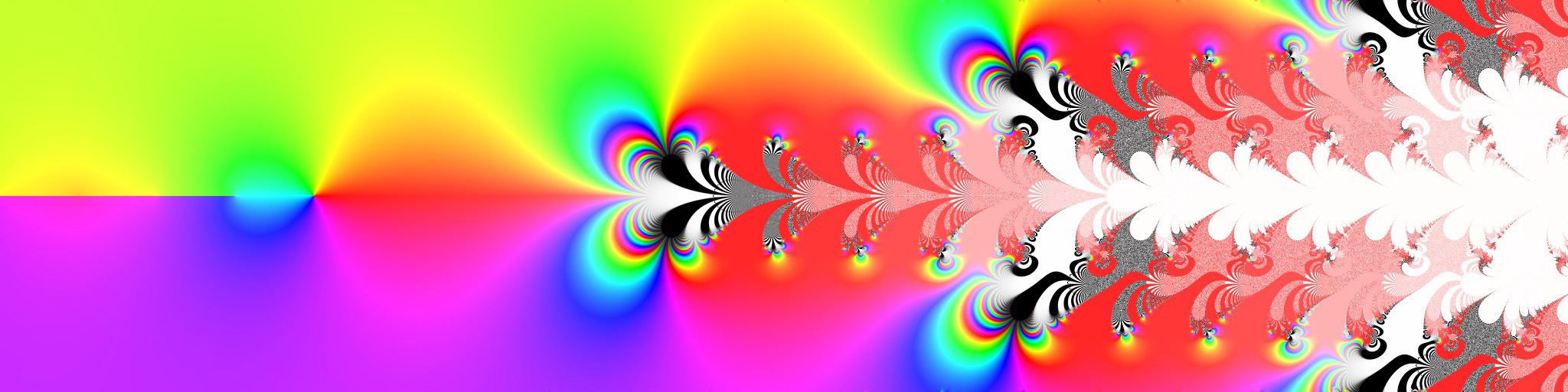 In grade school, we all learned the basic arithmetic operators: multiplication is repeated addition, and exponentiation is repeated multiplication. But not many have learned about hyper operators: tetration is repeated exponentiation, pentation is repeated tetration, and hexation is repeated pentation. For example, consider the tetration ze. When z = 3, we have 3e = eee. But what if z is not an integer, or what if z is complex? Nobody knows how to calculate the tetration in those cases, but we can make a good guess using Taylor series expansions. Shown here is an approximate plot of ze where z is a complex number. This plot uses coefficients from this C++ code by Dmitrii Kouznetsov. Notice that ze transitions into an iterated fractal system as z becomes large. Some people believe the study of tetration may eventually help to unify the branches of mathematics. Click here to download some Mathematica code.
Links Tetration - excellent article in Citizendium Tetration Forum - discussion forum Tetration.org - informative website, by Daniel Geisler Who can name the Biggest Number? - arrow notation, chained arrow notation, Busy Beavers Large Numbers |
Stereographic Projection of a Dodecahedron - POV-Ray, 10/10/08
 Here is a stereographic projection of a dodecahedron. This is the 3D counterpart to the 4D dodecaplex. Here is some Mathematica code:
(* runtime: 0.4 second *) z1 = (Sqrt[5] - 3)/Sqrt[30.0 - 6 Sqrt[5]]; z2 = Sqrt[(1 + 2/Sqrt[5])/3.0]; r1 = Sqrt[2(1 + 1/Sqrt[5])/3.0]; r2 = Sqrt[2(1 - 1/Sqrt[5])/3.0]; vertices = Join[Table[{r2 Cos[theta], r2 Sin[theta], z2}, {theta, 0, 2Pi - 0.4Pi, 0.4Pi}], Table[z1 = -z1; {r1 Cos[theta], r1 Sin[theta], z1}, {theta, 0, 1.8Pi, 0.2Pi}], Table[{r2 Cos[theta], r2 Sin[theta], -z2}, {theta, 0.2Pi, 1.8Pi, 0.4Pi}]]; edges = {{1, 2}, {2, 3}, {3, 4}, {4, 5}, {5, 1}, {1, 6}, {2, 8}, {3, 10}, {4, 12}, {5, 14}, {6, 7}, {7, 8}, {8, 9}, {9, 10}, {10, 11}, {11, 12}, {12, 13}, {13, 14}, {14, 15}, {15, 6}, {7, 16}, {9, 17}, {11, 18}, {13, 19}, {15, 20}, {16,17}, {17, 18}, {18, 19}, {19, 20}, {20, 16}}; Show[Graphics3D[Map[Line[vertices[[#]]] &, edges]]] norm[x_] := x.x; Normalize[x_] := x/Sqrt[x.x]; Rx[theta_] := {{1, 0, 0}, {0, Cos[theta], -Sin[theta]}, {0,Sin[theta], Cos[theta]}}; ProjectPoint[{x_, y_, z_}] := 2{x, y}/(1 - z); ProjectSegment[{v1_, v2_}] := Module[{p1 = ProjectPoint[v1], p2 = ProjectPoint[v2]}, {nx, ny, nz} = Normalize[Cross[v1, v2]]; If[nz != 0, p0 = -2{nx, ny}/nz; r = 2/Abs[nz]; theta = Sign[nz]Re[ArcCos[(p1 - p0).(p2 - p0)/Sqrt[norm[p1 - p0]norm[p2 - p0]]]], theta = 0]; If[Abs[theta] > 0.001, theta1 = ArcTan[p1[[1]] - p0[[1]], p1[[2]] - p0[[2]]]; theta2 = theta1 + theta; If[theta1 > theta2, t = theta1; theta1 = theta2; theta2 = t]; Circle[p0, r, {theta1, theta2}], Line[{p1, p2}]]]; Do[Show[Graphics[Map[ProjectSegment[Map[Rx[phi].# &, vertices[[#]]]] &, edges], PlotRange -> 6{{-1, 1}, {-1, 1}}, AspectRatio -> Automatic]], {phi, 0, 2Pi, Pi/18}]; |
Kluchikov’s Favorite Isosurface - C++ version: 7/8/09; Mathematica and MathGL3d version: 2/28/05
 An isosurface or implicit surface can be thought of as a 3D contour. The original equation for this isosurface is attributed to Alex Kluchikov. I found some beautiful POV-Ray renditions of this surface on Christoph Hormann’s web site so I decided to see if I could render it using my own ray tracer. Isosurfaces are commonly used for scientific visualizations. Here is some Mathematica code:
(* runtime: 25 seconds *) << MathGL3d`OpenGLViewer`; x1 = 0.125; y1 = 0.25Sin[2 Pi/3]; Kluchikov[x_, y_, z_, t1_,t2_] := Module[{r = Sqrt[x^2 + z^2] - 1.5, theta = ArcTan[z, x] + Pi/2,t, x2, y2}, t = 8theta/3 + t1; x2 = r Sin[t] + y Cos[t]; y2 = r Cos[t] - y Sin[t]; 0.33(((x2 + 0.25)^2 + y2^2)^(1/64) + ((x2 - x1)^2 + (y2 + y1)^2)^(1/64) + ((x2 - x1)^2 + (y2 - y1)^2)^(1/64)) + 0.01Sin[5theta + t2]]; Scan[MVContourPlot3D[Kluchikov[x, y, z, If[#, 0, Pi/3], If[#, 0, Pi]], {x, -2, 2}, {z, -2, 2}, {y, -0.5, 0.5}, Contours -> {0.945}, PlotPoints -> 100, ContourStyle -> {RGBColor @@ If[#, {0, 0, 1}, {1, 1, 1}]}, MVAlpha -> If[#, 0.5, 1], MVNewScene -> #, MVReturnValue -> None] &, {True, False}] MVPasteGraphics[]; If you do not wish to use the free MathGL3d package, you can use ImplicitPlot3D or ContourPlot3D, but it doesn’t look as nice: (* runtime: 80 seconds *) << Graphics`ImplicitPlot3D`; ImplicitPlot3D[Kluchikov[x, y, z, 0, 0] == 0.945, {x, -2.1, 2.1}, {z, -2.1, 2.1}, {y, -0.55, 0.55}, PlotPoints -> 100] (* runtime: 80 seconds *) << Graphics`ContourPlot3D`; ContourPlot3D[Kluchikov[x, y, z, 0, 0], {x, -2.1, 2.1}, {z, -2.1, 2.1}, {y, -0.55, 0.55}, Contours -> {0.945}, PlotPoints -> 12, ContourStyle -> {EdgeForm[]}] This is how you can make this surface in POV-Ray: // runtime: 7 minutes camera{location 4*y look_at 0 up y right x} light_source{4*y,1} #declare x1=1/8; #declare y1=sin(2*pi/3)/4; #declare Sqr=function(X) {X*X}; #declare theta=function{atan2(x,z)+pi/2}; #declare r=function{sqrt(x*x+z*z)-1.5}; #declare T=function(x,y,z,t1) {8*theta(x,y,z)/3+t1}; #declare x2=function(x,y,z,t1) {r(x,y,z)*sin(T(x,y,z,t1))+y*cos(T(x,y,z,t1))}; #declare y2=function(x,y,z,t1) {r(x,y,z)*cos(T(x,y,z,t1))-y*sin(T(x,y,z,t1))}; #macro Kluchikov(t1,t2,c) isosurface{function{0.33*(pow(Sqr(x2(x,y,z,t1)+1/4)+Sqr(y2(x,y,z,t1)),1/64)+pow(Sqr(x2(x,y,z,t1)-x1)+Sqr(y2(x,y,z,t1)+y1),1/64)+pow(Sqr(x2(x,y,z,t1)-x1)+Sqr(y2(x,y,z,t1)-y1),1/64))+0.01*sin(5*theta(x,y,z)+t2)-0.945} threshold 0 accuracy 0.0002 max_gradient 0.75 contained_by{box{-<2.1,0.55,2.1>,<2.1,0.55,2.1>}} pigment{rgbt c}} #end Kluchikov(0,0,<1,1,1,0>) Kluchikov(pi/3,pi,<0,0,1,0.5>) Link: Polygonising a scalar field - how to make metaballs, by Paul Bourke |
Belousov-Zhabotinsky (BZ) Reaction - Mathematica 4.2, 5/10/07
 This periodic cellular automaton simulates a chemical reaction called a Belousov-Zhabotinsky reaction. Here is some Mathematica code:
(* runtime: 24 seconds *) n = 50; SeedRandom[0]; image = Table[Random[Integer, {0, 255}], {n}, {n}]; Do[image = Table[z = image[[i, j]]; If[z == 255, 0, zlist = Flatten[image[[Mod[i - {0, 1, 2},n] + 1, Mod[j - {0, 1, 2}, n] + 1]]]; a = 9 - Count[zlist, 0]; If[z ==0, b = Count[zlist, 255]; Floor[(a - b)/3] + Floor[b/3], Min[Floor[Plus @@ zlist/a] + 45, 255]]], {i, 1, n}, {j, 1, n}]; ListDensityPlot[image, Mesh -> False, Frame -> False], {200}]; Links Mathematica notebook - by Takashi Yoshino Five Cellular Automata program - by Hermetic Systems |
Dual of the Geodesic Sphere - calculated in Mathematica 4.2, rendered in POV-Ray 3.6.1, 2/1/11
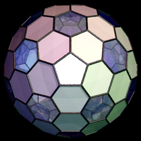
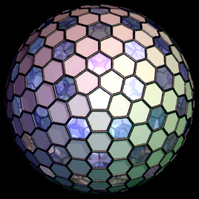 These geodesic spheres are inspired after Taff Goch's Hex-Pent Geodesic Sphere/Dome. The geodesic dome can be constructed by subdividing the triangular faces of an icosahedron into smaller triangles and projecting the vertices onto a dome. Then if you take the dual of the geodesic dome, you get a polyhedron composed entirely of pentagons and hexagons. But interestingly enough, no matter how many times you subdivided the geodesic dome, it's dual always has 12 pentagons. Another way to find a similar dual is to convert the triangles to hexagons and pentagons by removing central vertices. Buckminster Fuller patented the mathematics of the dome in 1954. Here is some Mathematica code:
(* runtime: 0.02 second *) Normalize[x_] := x/Sqrt[x.x]; Rx[theta_] := {{1, 0, 0}, {0, Cos[theta], -Sin[theta]}, {0, Sin[theta], Cos[theta]}}; Rz[theta_] := {{Cos[theta], -Sin[theta], 0}, {Sin[theta], Cos[theta], 0}, {0, 0, 1}}; ApplyMatrix[R_, plist_] := Map[R.# &, plist]; phi = (1 + Sqrt[5])/2; phi1 = ArcCos[Sqrt[(3 + 4 phi)/15]]; phi2 = ArcCos[Sqrt[(7 - 4 phi)/15]]; face = Table[{Cos[theta], Sin[theta], (phi + 1)/2}, {theta, Pi/6.0, 1.5 Pi, 2Pi/3}]; icosahedron = Table[{ApplyMatrix[Rz[theta].Rx[phi1].Rz[Pi], face], ApplyMatrix[Rz[theta].Rx[phi2], face], ApplyMatrix[Rz[theta + Pi/5].Rx[Pi - phi2].Rz[Pi], face], ApplyMatrix[Rz[theta + Pi/5].Rx[Pi - phi1], face]}, {theta,0, 1.6Pi, 0.4Pi}]; Subdivide[{p1_,p2_, p3_}] := Module[{p12 =p1 + p2, p23 = p2 + p3, p13 = p1 + p3}, Map[Normalize, {{p12, p23, p13}, {p1,p12, p13}, {p2, p23, p12}, {p3, p13, p23}}, {2}]]; Show[Graphics3D[Polygon /@ Join @@ Subdivide /@ Join @@Subdivide /@ Join @@ icosahedron]] Links Buckminsterfullerene (Buckyball) - truncated icosahedron arrangement of carbon atoms, same shape as a soccer ball, see this assembly movie Sphere Tessellation Icosahedron Subdivision - paper by Gernot Hoffmann Thomson Problem - Points on a Sphere - Java applet demonstrating minimum energy configuration of electrons on a sphere (Thomson problem), by Cris Cecka Magnus Wenninger - famous monk for creating origami polyhedrons |
Knots Within Knots - Mathematica 4.2, POV-Ray 3.6.1, 3/1/11
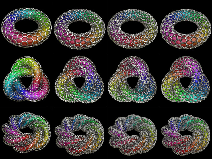 These knots are covered with networks of smaller knots.
Links Hexa Tube - sample Mathematica code for hexagonal tilings, by Mark McClure 8nov04b5 - trefoil weave by Robert Scharein |
Moiré Pattern - POV-Ray 3.6.1 version: 4/15/07, Mathematica 4.2 version: 1/29/05
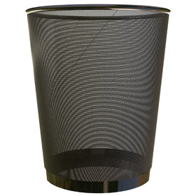
 A Moiré pattern is the interference of two similar overlapping patterns. Here is the Moiré pattern on a twisted IKEA wastepaper basket. The mesh on the wastepaper basket was ray-traced from 100,000 tiny cylinders. Here is some Mathematica code to plot Moiré contours around radiating lines:
(* runtime: 1.7 seconds *) f[dx_] := Sin[200ArcTan[x - dx, y]]; DensityPlot[f[0.1] - f[-0.1], {x, -1, 1}, {y, -1, 1}, PlotRange -> {0, 1}, PlotPoints -> 275, Mesh -> False, Frame -> False] |
 Here is some Mathematica code to plot a Moiré pattern from rapidly varying contours of a function:
(* runtime: 0.8 second *) f[z_] := z^3; DensityPlot[Sin[20Pi Abs[f[x + I y]]], {x, -2.5, 2.5}, {y, -2.5, 2.5}, PlotPoints -> 275, Mesh -> False, Frame -> False] Link: Mandelbrot Set Moire Pattern - by Bernard Helmstetter |
Dodecahedron Costume - Cricut Explore One, 10/29/17
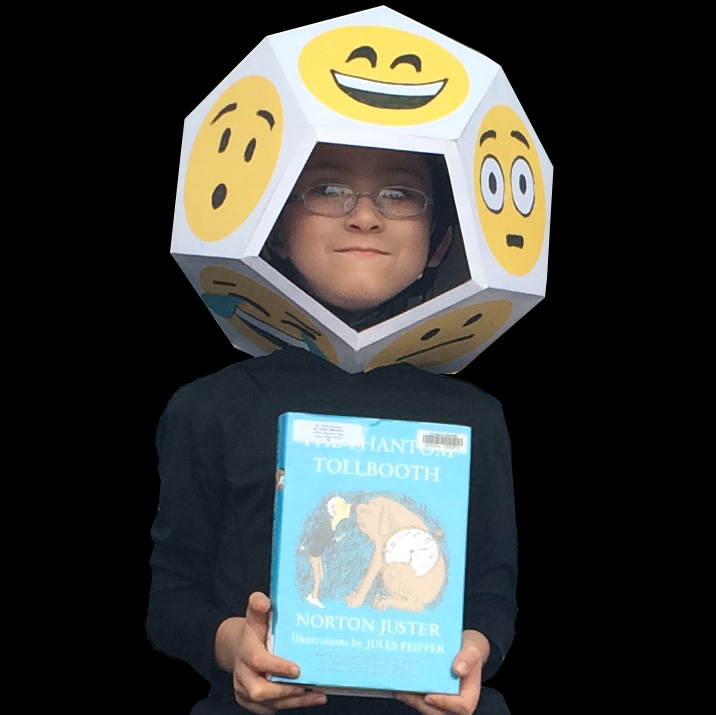
 This dodecahedron costume was inspired after the Dodecahedron character in Norton Juster's popular book, The Phantom Tollbooth. We cut it out of carboard using the Cricut Explore One knife dragging CNC cutting machine.
 |
Spherical Canvas versus Reflective Sphere - POV-Ray 3.6.1, 10/17/07
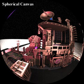
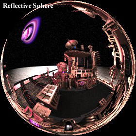

 This image was inspired by Dick Termes' paintings of 3D worlds on a spherical “canvas” called Termespheres. These images have 6 vanishing points as opposed to linear perspective drawings which only have 3 vanishing points. The left picture shows my version of a spherical canvas for my factory scene. This was accomplished by rendering a spherical panorama of the scene in POV-Ray, and then mapping it to a sphere. Click here to download some sample POV-Ray code. The right picture shows a reflective sphere when viewed from the exact same position. As you can see, it looks quite different.
 |
Torus Knots - Mathematica 4.2, MathGL3d, POV-Ray 3.6.1, 10/31/04
 This is one continuous torus knotted on itself. The left image shows a (11,3) torus knot and the right image shows a (6,13) torus knot. This image was featured on the cover of McGraw-Hill's 2012 Pre-Calculus textbook. Click here to see a rotatable 3D version. Click here to download an animated screensaver along with C++ source code. Click here to download some POV-Ray code for this image. The following Mathematica code was adapted from Maxim Rytin’s TubePlot code:
(* runtime: 2.6 seconds *) Normalize[x_] := x/Sqrt[x.x]; p[t_] := {(1 + 0.3 Cos[11t/3])Cos[t], (1 + 0.3 Cos[11t/3]) Sin[t], 0.3 Sin[11t/3]}; f[t_, theta_] := Module[{dp = p'[t], ddp = p''[t], tangent, normal1, normal2},tangent = Normalize[dp]; normal1 = Normalize[ddp(dp.dp) - dp(dp.ddp)]; normal2 = Cross[tangent, normal1]; p[t] + 0.1 (normal1 Cos[theta] + normal2 Sin[theta])]; ParametricPlot3D[Append[f[t, theta], {EdgeForm[], SurfaceColor[Hue[t/(2Pi)]]}], {t,0, 6Pi}, {theta, 0, 2Pi}, PlotPoints -> {360, 15}, Compiled -> False] POV-Ray has an internal function for torus knots: // runtime: 8 seconds camera{location 16*y look_at 0} light_source{16*y,1} #declare f=function{internal(24)} isosurface{function{f(x,y,z,6,11,3,0.1,0.5,1,0.1,1,1,0)} max_gradient 2 contained_by{sphere{0,8}} pigment{rgb 1}} Knots Links Torus Knot Fun - animated torus knot by Krzystof Gears Trefoil - by Michael Trott Tubes and Knots - Mathematica code by Mark McClure One ring to rule the ball - 3D printed torus knot with ball, by TerraCotta |
Silver Spirals - AutoCAD 2000, POV-Ray 3.6.1, 8/19/02
 These are just some doodles I made while playing around with AutoCAD.
 |
Silver Noodles - AutoCAD 2000, POV-Ray 3.6.1, 11/30/10
 This is another doodle I made while playing around with AutoCAD.
 |
Intersection of 3 Cylinders - POV-Ray 3.6.1, 12/15/08
 One thing that has always intrigued me is the intersection of three perpendicular cylinders all meeting at the same point. Notice that the resulting shape is not a sphere. In fact, when viewed from a certain angle, the outline of this shape looks like a hexagon.
 |
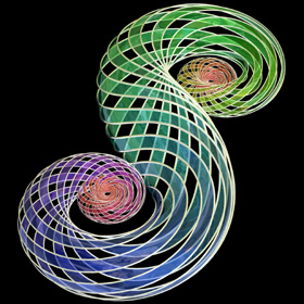
Loxodrome - POV-Ray 3.6.1, 10/2/08
 A Loxodrome (or Rhumb line) is a spherical spiral. A ship takes this path when it maintains a constant angle with respect to the equator. This image shows a loxodrome intertwined with spirals.
Links Rhombic Triacontahedron IV - sculpture composed of loxodromes, by Vladimir Bulatov, see also his pendant Loxodromic Fractal World - by Ramiro Perez |
Golden Ratio Logarithmic Spiral Transformation - Mathematica 4.2, 6/21/04
 The Golden Ratio f = (1 + sqrt(5))/2 ≈ 1.61803 has an interesting relationship with Fibonacci Numbers. The basic equation for a Golden Spiral is given by r(q) = f2q/p. The interlocking rings pattern in this image was adapted from M. C. Esher’s Snakes. Here is some Mathematica code:
(* runtime: 48 seconds *) image = Import["C:/Picture.jpg"][[1, 1]]/255.0; imax = Length[image]; jmax = Length[image[[1]]]; n = 275; phi = 0.5 (1 + Sqrt[5]); Show[Graphics[RasterArray[Table[Module[{x = 2j/n - 1, y = 2i/n - 1, r, theta}, r = x^2 + y^2; theta = ArcTan[y, x]; RGBColor @@ If[r != 0, image[[Floor[imax Mod[2theta/Pi, 1]] + 1, Floor[jmax Mod[theta/Pi + 0.25Log[r]/Log[phi], 1]] + 1]], {0, 0, 0}]], {i, 1, n}, {j, 1, n}]], ImageSize -> n, PlotRange -> {{0, n}, {1, n}}, AspectRatio -> 1]] Links Droste Effect Gallery - recursive pictures by Josh Sommers Seamless Maker - Droste effect software by Hypatiasoft |
Complex Map Polar Transformation: f(z) = e2 p z - Mathematica 4.2, 6/14/04
 These images were generated by mapping a tessellation to the complex plane, similar to M. C. Esher’s Development II. Here is some Mathematica code:
(* runtime: 80 seconds *) image = Import["Picture.jpg"][[1, 1]]; n = Length[image]; m = Length[image[[1]]]; Show[Graphics[RasterArray[Table[RGBColor @@ Module[{z = Log[2j/275 - 1 + I (2i/275 - 1)]/(2Pi) + 1.0}, image[[Floor[n Mod[6 m Re[z]/n, 1]] + 1, Floor[m Mod[6 Im[z], 1]] + 1]]/255.0], {i, 1, 275}, {j, 1, 275}]], ImageSize -> 275, PlotRange -> {{0, 275}, {1, 275}}, AspectRatio -> 1]] |
Fisheye Transformation - Mathematica 4.2, 6/15/04
 Here is some Mathematica code:
(* runtime: 26 seconds *) image = Import["C:/Picture.jpg"][[1, 1]]; n = Length[image]; m = Length[image[[1]]]; Show[Graphics[RasterArray[Table[RGBColor @@ Module[{x = 2j/275 - 1, y = 2i/275 - 1, r, h}, r = 1.0 - x^2 - y^2; h = 0.5(1 - 0.5If[r > 0, Sqrt[r], 0]); image[[Floor[n Mod[5 m h x/n, 1]] + 1, Floor[m Mod[5 h y, 1]] + 1]]/255.0], {i, 1, 275}, {j, 1, 275}]], ImageSize -> 275, PlotRange -> {{0, 275}, {1, 275}}, AspectRatio -> 1]] |
RSA Encryption (Rivest, Shamir and Adleman) - Mathematica 4.2, 11/15/06
|
Here is some Mathematica code to encrypt messages using prime numbers. Anyone with the public key (and n) can encode messages, but only the person with the secret key can decode them: (* runtime: 0.05 second *) message = "This is a secret message containing 112 characters. This message will be divided into 4 blocks of 28 characters."; << NumberTheory`NumberTheoryFunctions`; SeedRandom[0]; PublicKey = NextPrime[Random[]256^28]; p = NextPrime[Random[]256^14]; q = NextPrime[256.0^28/p]; n = p q; SecretKey = PowerMod[PublicKey, -1, (p - 1)(q - 1)]; ToNumbers[str_] := Map[FromDigits[#, 256] &, Partition[ToCharacterCode[str], 28]]; ToText[nlist_] := StringJoin @@ Map[StringJoin @@ Map[FromCharacterCode, IntegerDigits[#, 256, 28]] &, nlist]; encryption = ToText[Map[PowerMod[#, PublicKey, n] &, ToNumbers[message]]] ToText[Map[PowerMod[#, SecretKey, n] &, ToNumbers[encryption]]] If you do not know p and q, you can try to break the code using this method (but it is very slow): (* runtime: 40 minutes *) SecretKey = PowerMod[PublicKey, -1, EulerPhi[n]]; Here’s a basic idea how these functions work: InverseMod[a0_, n0_] := Module[{n = n0, a = a0, x = 0, x1 = 0,x2 = 1, q1 = 0, q2 = 0, i = 1}, While[a != 0, If[i > 2, x = Mod[x1 - x2 q1 + n0^2, n0]; x1 = x2; x2 = x]; q1 = q2; q2 = Floor[n/a]; {n, a} = {a, Mod[n, a]}; i++]; Mod[x1 - x2 q1 + n0^2, n0]]; PowerMod[a_, b_, n_] := If[b == -1, InverseMod[a, n], Module[{c = 1}, digits =IntegerDigits[b, 2]; Scan[If[#[[1]] == 1, c = Mod[c #[[2]], n]] &, Transpose[{digits, Reverse[NestList[Mod[#^2, n] &,a, Length[digits] - 1]]}]]; c]]; GCD[a_, b_] := If[b == 0, a, GCD[b, Mod[a, b]]]; Link: RSA Encryption - Mathematica notebook by Kit Dodson |
Spirographs - MacDraw (vector art), 1992?
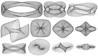 I made these a very long time ago on my old Macintosh. I don’t remember how to make them anymore.
 |
Mathematica Typesetting Shortcuts
Here is a Mathematica notebook that summarizes some convenient Mathematica typesetting shortcuts. You can type equations quite quickly in Mathematica once you know these shortcuts. I use these shortcuts to type my class notes in Mathematica.
Mathematica Links
Mathematica - excellent technical computing software, easy to make beautiful plots and play equations as sounds
MathGL3d - free Mathematica package for rendering with OpenGL and writing POV-Ray scripts
LiveGraphics3D - software for displaying rotatable 3D Mathematica graphics on the internet
JavaView - another program similar to LiveGraphics3D
Mathematica Information Center - many sample notebooks & packages
Mathematica Art - I especially like the animated GIFs
Mathematicians
The Thirty Greatest Mathematicians - interesting biographies by James Dow Allen
Leonhard Euler - had a photographic memory, did his greatest work after he went blind, saying "Now I will have less distraction"
Carl Gauss - perhaps the greatest mathematician who ever lived, corrected his family finances at the age of 3
Srinivasa Ramanujan - self-taught mathematician who grew up in poverty and baffled leading mathematicians, developed amazing formulas for pi
Évariste Galois - proved there is no quintic formula, died in a duel at age 20 over a woman
Andrew Wiles - solver of Fermat's Last Theorem
John Nash - the movie "A Beautiful Mind" is based on his life
Other Math Links
Paul Nylander's Page - at the Virtual Art Museum
Game Puzzles - math art puzzles & games, by Kate Jones
Sphere Eversion - beautiful animation turning a sphere inside-out by Bill Thurston
Penrose Tiling - amazing aperiodic tilings discovered by Roger Penrose, here is a Mathematica notebook by E. Arthur Robinson
Hyperseeing - electronic publication by The International Society of the Arts, Mathematics, and Architecture
Chatin’s Constant - the infamous “incalculable” constant, the probability that a random algorithm halts
Fractional Calculus - fractional derivatives
Strang’s Strange Figures - unexpected patterns in trig functions
Wikipedia article on p
Gödel's Incompleteness Theorem - famous paper that supposedly defeats all hope of formally proving all truth. I can’t say I understand it, but it’s interesting (and controversial).
Chinese Rings - a simple puzzle that can be solved in no less than 18446744073709551616 moves
Number Spiral - interesting pattern of prime numbers
echochrome - M.C. Escher video game
Probability theory paradoxes - Monty Hall problem, Simpson's paradox
The Math Book - by Clifford Pickover, includes some of my math artwork
Rose windows - beautiful stained glass windows found in Gothic churches