Potential Flow

Potential Flow
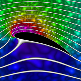
A potential flow is characterized by any flow where the velocity is irrotational. Here are some useful formulas for potential flow:

Here is a summary of some basic flows used in potential flow calculations:

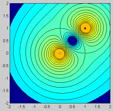
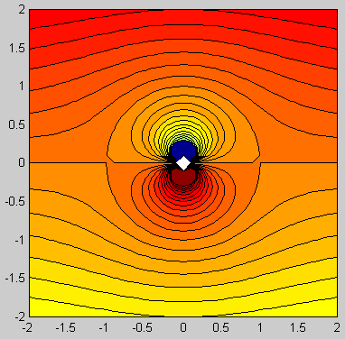
Vortex Outside Cylinder

Vortex Outside Cylinder.

Matlab code:
gamma=1; a=1; Z=1+1i;
xlist=-2:0.04:2; [x,y]=meshgrid(xlist,xlist); z=x+1i*y;
w=1i*gamma/(2*pi)*(-log(z-Z)+log(a^2./z-conj(Z)));
contourf(xlist,xlist,imag(w),-0.1:0.02:0.2); axis square;

Mathematica code:
gamma = a = 1; Z = 1 + I; w[z_] := (I gamma/(2Pi))(-
Log[z - Z] + Log[a^2/z - Conjugate[Z]]);
ContourPlot[Im[w[x + I y]], {x, -2.0, 2.0}, {y, -2.0, 2.0}, Contours -> Table[psi, {psi, -0.1, 0.2, 0.02}], PlotPoints -> 100, ContourShading -> False, AspectRatio -> Automatic];

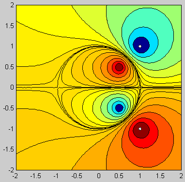
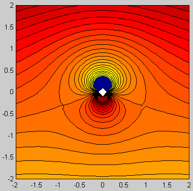
Two Vortices Outside Cylinder

Two Vortices Outside Cylinder.

Matlab code:
gamma=1; a=1; ZA=1+1i; ZB=conj(ZA);
xlist=-2:0.04:2; [x,y]=meshgrid(xlist,xlist); z=x+1i*y;
w=1i*gamma/(2*pi)*(log((z-ZA)./(z-ZB))-log((z-a^2/ZB)./(z-a^2/ZA)));
contourf(xlist,xlist,imag(w),0.25*(-1:0.125:1).^3); axis square;

Mathematica code:
gamma = a = 1; ZA = 1 + I; ZB = Conjugate[ZA]; w[z_] := (I gamma/(2Pi))(Log[(z - ZA)/(z - ZB)] - Log[(z - a^2/ZB)/(z - a^2/ZA)]);
ContourPlot[Im[w[x + I y]], {x, -2.0, 2.0}, {y, -2.0, 2.0}, Contours -> Table[0.25psi^3, {psi, -1.0, 1.0, 0.125}], PlotPoints -> 100, ContourShading ->False, AspectRatio -> Automatic];

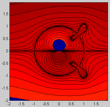
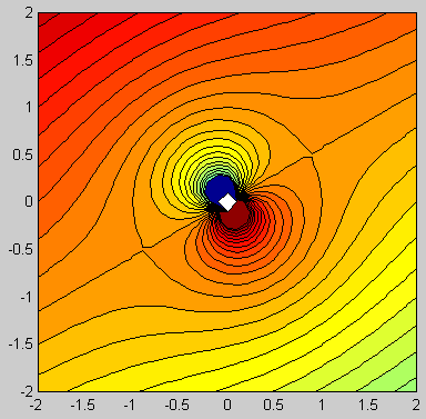
Cylinder with Outside Vortices

Cylinder with Outside Vortices.

Matlab code:
gamma=1; a=1; ZA=1+1i; ZB=conj(ZA); rA=abs(ZA); U=gamma*rA^5/a^5/((rA^2/a^2-1)^2*(rA^2/a^2+1)^2);
xlist=-2:0.06:2; [x,y]=meshgrid(xlist,xlist); z=x+1i*y;
w=U*(z+a^2./z)+1i*gamma/(2*pi)*(log((z-ZA)./(z-ZB))-log((z-a^2/ZB)./(z-a^2/ZA)));
contourf(xlist,xlist,imag(w),(-1:0.1:1).^3); axis square;

Mathematica code:
gamma = a = 1; ZA = 1 + I; ZB = Conjugate[ZA]; rA = Abs[ZA]; U = (gamma rA^5/a^5)/((rA^2/a^2 - 1)^2(rA^2/a^2 + 1)^2);
w[z_] := U(z + a^2/z) + (I gamma/(2Pi))(Log[(z - ZA)/(z - ZB)] - Log[(z - a^2/ZB)/(z - a^2/ZA)]);
ContourPlot[Im[w[x + I y]], {x, -2, 2}, {y, -2,2}, Contours -> Table[psi^3, {psi, -1.0, 1.0, 0.1}], PlotPoints -> 100, ContourShading -> False, AspectRatio -> Automatic];

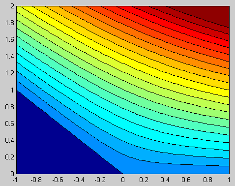
Corner Flow

Corner Flow.

Matlab code:
A=1; beta=3*pi/4;
xlist=-1:0.04:1; ylist=0:0.04:2; [x,y]=meshgrid(xlist,ylist); z=x+1i*y;
w=A*z.^(pi/beta);
contourf(xlist,ylist,imag(w),0:0.125:2.5);

Mathematica code:
A = 1; beta = 3Pi/4; alpha = Pi/beta; w[z_] := A z^alpha;
ContourPlot[Im[w[x + I y]], {x, -1, 1}, {y, 0, 2}, Contours -> Table[psi, {psi, 0, 2.5, 0.125}], PlotPoints -> 100,ContourShading -> False, AspectRatio -> Automatic];

Cylinder

Cylinder.

Matlab code:
U=1; a=1; xlist=-2:0.1:2; [x,y]=meshgrid(xlist,xlist); z=x+1i*y; w=U*(z+a^2./z);
contourf(xlist,xlist,imag(w),-3:0.25:3); axis square;

Mathematica code:
U = a = 1; w[z_] := U(z + a^2/z);
ContourPlot[Im[w[x + I y]], {x, -2, 2}, {y, -2,2}, Contours -> Table[psi, {psi, -3, 3, 0.25}], PlotPoints -> 100, ContourShading -> False, AspectRatio -> Automatic];

Lifting Cylinder

Lifting Cylinder.

Matlab code:
U=1; gamma=4; a=1; xlist=-2:0.1:2; [x,y]=meshgrid(xlist,xlist); z=x+1i*y;
w=U*(z+a^2./z)+1i*gamma/(2*pi)*log(z);
contourf(xlist,xlist,imag(w),-3:0.25:3); axis square;

Mathematica code:
U = 1; gamma = 4; a = 1; w[z_] := U(z + a^2/z) + (I gamma/(2Pi))Log[z];
ContourPlot[Im[w[x + I y]], {x, -2, 2}, {y, -2, 2}, Contours -> Table[psi, {psi, -3, 3, 0.25}], PlotPoints -> 100, ContourShading -> False, AspectRatio -> Automatic];

Cylinder with Angle of Attack

Cylinder with Angle of Attack.

Matlab code:
alpha=pi/6; U=1; a=1; xlist=-2:0.1:2; [x,y]=meshgrid(xlist,xlist); z=x+1i*y;
w=U*(z*exp(-1i*alpha)+a^2./(z*exp(-1i*alpha)));
contourf(xlist,xlist,imag(w),-3:0.25:3); axis square;

Mathematica code:
alpha = Pi/6; U = 1; a = 1; w[z_] := U(z Exp[-I alpha] + a^2/(z Exp[-I alpha]));
ContourPlot[Im[w[x + I y]], {x, -2, 2}, {y, -2, 2}, Contours -> Table[psi, {psi, -3, 3, 0.25}], PlotPoints ->100, ContourShading -> False, AspectRatio -> Automatic];

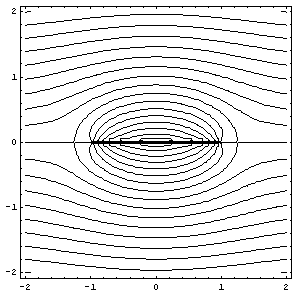
Rankine Oval

Rankine Oval.

Mathematica code:
U = 1; a = 1; b = 0.5; zeta[z_] := (z + Sign[Re[z]]Sqrt[z^2 - 4 b^2])/2 ; w[z_] := U(zeta[z] + a^2/zeta[z]);
ContourPlot[Im[w[x + I y]], {x, -2, 2}, {y, -2,2}, Contours -> Table[psi, {psi, -2, 2, 0.2}], PlotPoints -> 100, ContourShading -> False, AspectRatio -> Automatic];

Joukowski Airfoil

Joukowski Airfoil (Rankine Oval that has been pinched by a translation in the zeta plane, lift and angle of attack added).

Mathematica code:
U = rho = 1; chord = 4; thk = 0.5; alpha = Pi/9; y0 = 0.2; x0 = -thk/5.2; L = chord/4; a = Sqrt[y0^2 + L^2]; beta = ArcCos[L/a]; gamma = 4Pi rho U^2a (alpha + beta);w[z_] := Module[{zeta = (z +sign Sqrt[z^2 - 4 L^2])/2}, zeta = (zeta - x0 - I y0)Exp[-I alpha]/Sqrt[(1 - x0)^2 + y0^2]; U(zeta + a^2/zeta) + (I gamma/(2Pi)) Log[zeta]]; w2[z_] = w[z] /. sign -> Sign[Re[z]];
ContourPlot[Im[w2[(x + I y)Exp[I alpha]]], {x, -3, 3}, {y, -3, 3}, Contours -> Table[x^3 + 0.0208, {x, -1, 1, 0.1}], PlotPoints -> 100, ContourShading -> False, AspectRatio -> Automatic];

Schwarz Christoffel Source

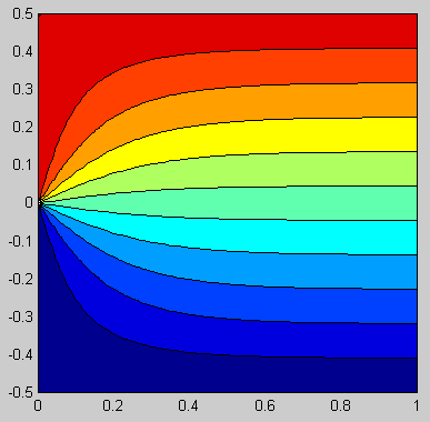
Schwarz Christoffel Source.

Matlab code:
U=1; h=1; m=2*h*U;
xlist=0:0.01:1; ylist=-0.5*h:0.01*h:0.5*h; [x,y]=meshgrid(xlist,ylist); z=x+1i*y;
w=m/(2*pi)*log(1i*sinh(pi*z/h));
contourf(xlist,ylist,imag(w),10); axis square;

Mathematica code:
U = h = 1; m = 2h U; w[z_] := (m/(2Pi))Log[I Sinh[Pi z/h]];
ContourPlot[Im[w[x + I y]], {x, 0, 1}, {y, -0.5h, 0.5h}, Contours -> 10, PlotPoints -> 100, ContourShading -> False, AspectRatio -> Automatic];

Schwarz Christoffel Step

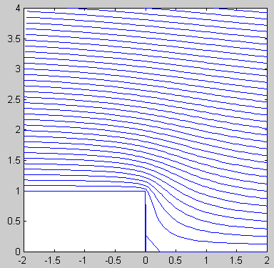
Schwarz Christoffel Step.

Matlab code:
U=1; h=1; phi=-3.01:0.05:2;
for psi=0:0.1:3.5;
w=phi+1i*psi; zeta=w/(h*U/pi); sign1=sign(real(w));
z=(h/pi)*(sign1.*sqrt(zeta.^2-1)+log(zeta+sign1.*sqrt(zeta.^2-1)));
if(psi==0); hold off; else; hold on; end;
plot(real(z),imag(z));
end;
axis([-2 2 0 4]); axis square; hold off;

Mathematica code:
<< Graphics`Master`; ToPoint[z_] := {Re[z], Im[z]};
U = h = 1; zeta = w/(h U/Pi); sign = Sign[Re[w]]; z[w_] = (h/Pi)(sign Sqrt[zeta^2 - 1] + Log[zeta + sign Sqrt[zeta^2 - 1]]);
DisplayTogether[Table[ParametricPlot[ToPoint[z[phi + I psi]], {phi, -4, 2}, Compiled -> False], {psi, 0, 3.5, 0.1}], AxesLabel -> {"x", "y"}, PlotRange -> {{-2, 2}, {0, 4}}, AspectRatio -> Automatic];

Leap-Frogging

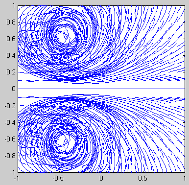
Solves Euler’s equations (inviscid flow) and plots the pathlines. The vortex effects are found using the Biot-Savart law. The differential equations are solved using the Adams Bashforth method.

Matlab code:
dt=0.01; rcore=0.1; dz0=0; Klist=[1,-1,1,-1];
zlist=[-1-0.5i,-1+0.5i,-0.5-0.5i,-0.5+0.5i]; i=length(Klist)+1;
for x=-1:0.1:1; for y=-1:0.1:1; zlist(i)=x+1i*y; i=i+1; end; end;
n=length(zlist);
for i=1:n; for j=1:10; paths(i,j)=zlist(i); end; end;
for t=1:85;
for i=1:n; dz(i)=0; for j=1:length(Klist); if(zlist(i)!=zlist(j)); r2=abs(zlist(i)-zlist(j))^2;
dz(i)=dz(i)+1i*Klist(j)*(zlist(j)-zlist(i))/r2*(1-exp(-r2/rcore^2));
end; end; end;
zlist=zlist+dt*(1.5*dz-0.5*dz0); dz0=dz;
hold on;
for i=1:n; temp=cat(2,zlist(i),paths(i,:)); temp(11)=[]; paths(i,:)=temp;
plot(real(temp),imag(temp));
end;
axis([-1,1,-1,1]); axis square; hold off;
end;

Mathematica code:
(* runtime: 19 seconds *)
ToPoint[z_] := {Re[z], Im[z]};dt = 0.01; rcore = 0.1; dz0 = 0; Klist = {1, -1, 1, -1};
zlist = Join[{-1 - 0.5I, -1 + 0.5I, -0.5 - 0.5I, -0.5 + 0.5I}, Flatten[Table[x + I y, {x, -1, 1, 0.1}, {y, -1, 1, 0.1}], 1]];
paths = Map[# Table[1, {10}] &, zlist];
Do[dz = Map[Sum[zj = zlist[[j]]; If[# != zj, r2 = Abs[# - zj]^2; I Klist[[j]](zj - #)/r2 (1 -Exp[-r2/rcore^2]), 0], {j, 1, Length[Klist]}] &, zlist]; zlist += dt (1.5dz - 0.5dz0); dz0 = dz; paths = Table[Prepend[Delete[paths[[i]], -1], zlist[[i]]], {i, 1, Length[zlist]}];Show[Graphics[Map[Line[Map[ToPoint, #]] &, paths], PlotRange -> {{-1, 1}, {-1, 1}}, AspectRatio -> Automatic]], {85}];

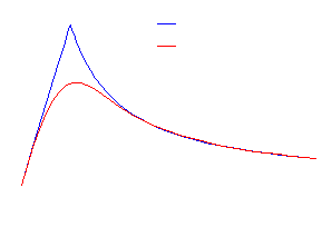
Here is the difference between linearly decaying vortices and vortex blobs: