


I think fractals are one of the most interesting puzzles of mathematics. Many fractals can be made by a simple formula, yet they have such beautiful and complex designs. This page provides simple Mathematica code for many of the most interesting types of fractals. Some of this code may not be very efficient, but it should be enough to give you a basic understanding of the mathematics involved.
Kleinian Double 1/15 Cusp Group - calculated in Mathematica 4.2, rendered in POV-Ray 3.6.1, 8/10/05
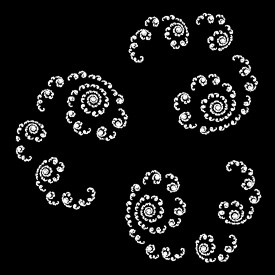
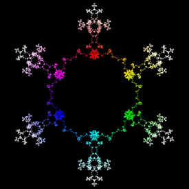
 Here is my attempt to recreate the 1/15 double cusp group on page 269 of Indra’s Pearls. Click here to see some POV-Ray code and here for some AutoLisp code. You can also see this code on Roger Bagula’s web site. Here is some Mathematica code:
(* runtime: 0.03 second *) ta = 1.958591030 - 0.011278560I; tb = 2; tab = 0.5(ta tb - Sqrt[ta^2tb^2 - 4(ta^2 + tb^2)]); z0 = (tab - 2)tb/(tb tab - 2ta + 2I tab); a = {{ta/2, (ta tab - 2tb + 4I)/(2tab + 4)/z0}, {(ta tab - 2 tb - 4I)z0/(2tab - 4), ta/2}}; A = Inverse[a]; b = 0.5{{tb - 2I, tb}, {tb, tb + 2I}}; B = Inverse[b]; ToMatrix[{z_, r_}] := I{{z, r^2 - z Conjugate[z]}, {1, -Conjugate[z]}}/r; Fix[{{a_, b_}, {c_, d_}}] := 0.5(a - d - Sqrt[4 b c + (a - d)^2])/c; a1 = a.a.a.a.a.a.a.a.a.a.a.a.a.a.a.B; a2 = a.b.A.B; c1 = ToMatrix[{0, -1}]; c2 = ToMatrix[{x + I y, r} /. Solve[Map[(Re[#] - x)^2 + (Im[#] -y)^2 == r^2 &, {Fix[a1], Fix[a2], Fix[a1.a2]}], {x, y, r}][[2]]]; Reflect[c_, a_] := a.c.Inverse[Conjugate[a]]; orbits = Join[Reverse[NestList[Reflect[#, a] &, c1, 3*15 + 8]], Drop[NestList[Reflect[#, A] &, c1, 3*15 + 6], 1], Reverse[NestList[Reflect[#, a] &, c2, 3*15 - 7]], Drop[NestList[Reflect[#, A] &, c2, 3*15 + 7],1]]; Show[Graphics[Table[{{a, b}, {c, d}} = orbits[[i]]; {Hue[i/15], Disk[-{Re[a/c], Im[a/c]}, Re[I/c]]}, {i, 1, Length[orbits]}]], AspectRatio -> Automatic, PlotRange -> All] |


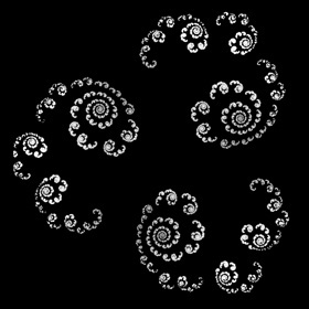
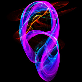
 Here is the inverse of the above group. The right animation shows the set morphing into a single cusp group. You can purchase this as a poster here.
Links Explanation - by David Wright, coauthor of Indra’s Pearls Kleinian Gallery - beautiful Kleinian groups by Jos Leys Doyle spirals - hexagonal circle packings by Jos Leys Limit Sets - interesting animations by Jeffrey Brock, see his 3D bending Gallery - includes some nice Kleinian groups, by Curtis McMullen Double Spiral - POV-Ray rendering by Jeffrey Pettyjohn Kreistiefe - hexagonal circle packings Java applet, by Tim Hoffmann and Nadja Kutz Swirlique - program for drawing Kleinian limit sets, by Terry Gintz Travelling Through Planets - animation, by Mehrdad Garousi |
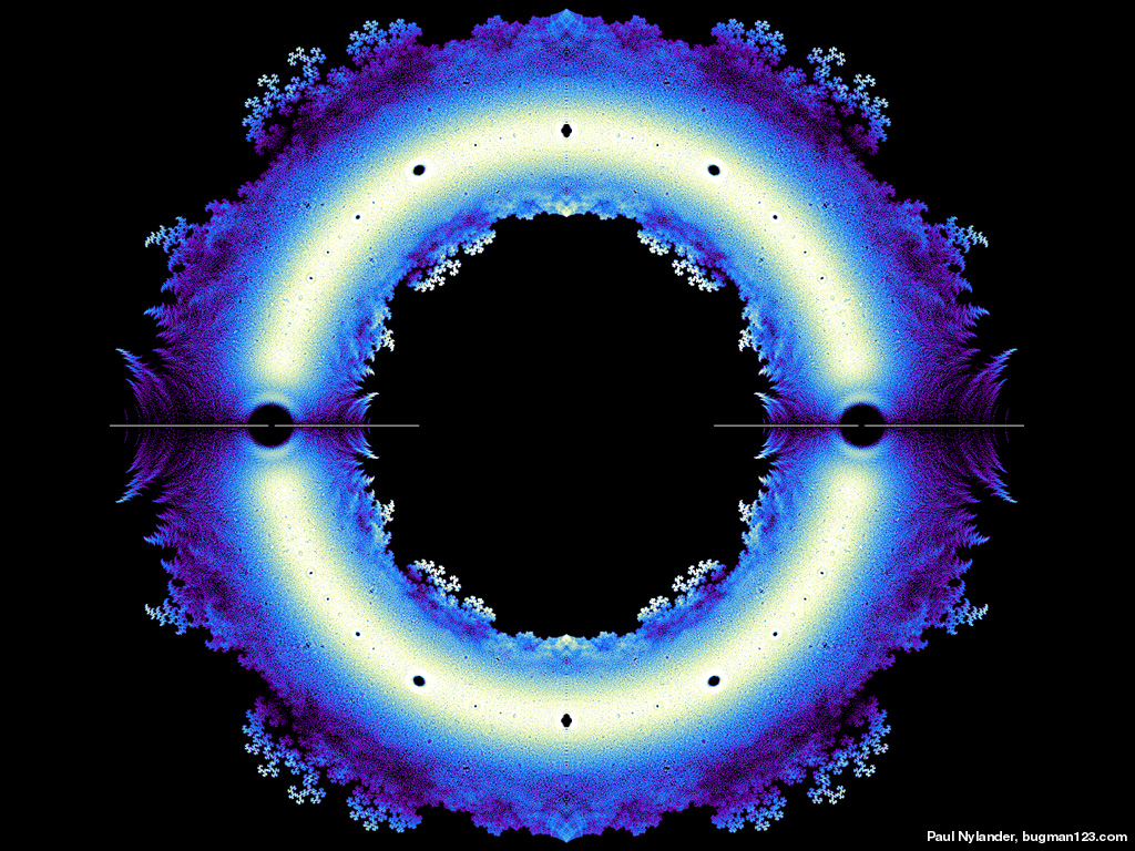
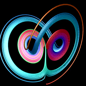
Kleinian Quasifuchsian Limit Set - new version: C#, old version: Mathematica 4.2, POV-Ray 3.6.1, 4/15/06
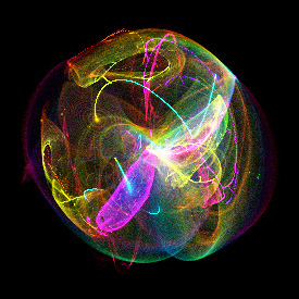
 Here is a butterfly “blown about” inside a Quasifuchsian limit set (see Fuchsian group). Originally, Felix Klein described these fractals as “utterly unimaginable”, but today we can visualize these fractals with computers. You can purchase this as a poster here. Here is some Mathematica code:
(* runtime: 12 seconds *) ta = tb = 1.91 + 0.05I; tab = (ta tb + Sqrt[ta^2tb^2 - 4(ta^2 + tb^2)])/2; z0 = (tab - 2)tb/(tb tab - 2ta + 2I tab); b = {{tb - 2I, tb}, {tb, tb + 2I}}/2; B = Inverse[b]; a = {{tab, (tab - 2)/z0}, {(tab + 2)z0, tab}}.B; A = Inverse[a]; homography[{{a_, b_}, {c_, d_}}, z_] := (b + a z)/(d + c z); ReflectList[C_, zlist_] := homography[C, #] & /@zlist; Children[zlist_] := ReflectList[#, zlist] & /@ {a, b, A, B}; zlist = {0.23 + 0.03 I, 0.18 + 0.05 I, 0.62 + 0.45 I, 0.86 + 0.73 I, 0.91 + 0.89 I, 0.88 + 0.97 I, 0.75 + 0.98 I, 0.48 + 0.88 I, 0.25 + 0.85 I, 0.04 + 0.79 I, -0.02 + 0.67 I, -0.1 + 0.78 I, -0.14 + 0.77 I, -0.24 + 0.84 I, -0.24 + 0.77 I, -0.41 + 0.88 I, -0.39 + 0.77 I, -0.5 + 0.82 I, -0.48 + 0.74 I, -0.82 + I, -0.86 + 0.96 I, -0.68 + 0.79 I, -0.7 + 0.74 I, -0.89 + 0.81 I, -0.74 + 0.64 I, -0.77 + 0.6 I, -0.91 + 0.65 I, -0.8 + 0.51 I, -0.87 + 0.44 I, -0.71 + 0.32 I, -0.44 + 0.19 I, -0.07 + 0.08 I, -0.38 + 0.03 I}; zlists1 = zlists2 = {0.5 + 0.125Join[Reverse[Conjugate[zlist]], zlist]}; test[zlist1_, zlist2_] := Abs[zlist2[[1]] - zlist1[[1]]] < 0.05; While[zlists2 =!= {},zlists2 = Complement[Flatten[Children /@ zlists2, 1], zlists1, SameTest -> test]; zlists1 = Union[zlists2, zlists1, SameTest -> test]]; Show[Graphics[Line[{Re[#], Im[#]} & /@ #] & /@ zlists1], AspectRatio -> Automatic] Links 3D Limit Set - amazing 3D Quasifuchsian limit set, by Keita Sakugawa (advisor Kazushi Ahara) 3D Quasifuchsian Fractals - created by reflecting sphairahedrons (spherical polyhedrons), by Kazushi Ahara and Yoshiaki Araki, see the gallery and video article on 3D hyperbolic tilings - by Vladimir Bulatov orbital Kleinian group fractals - created with Ross Hilbert's program Fractal Science Kit |
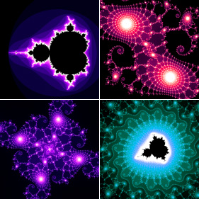
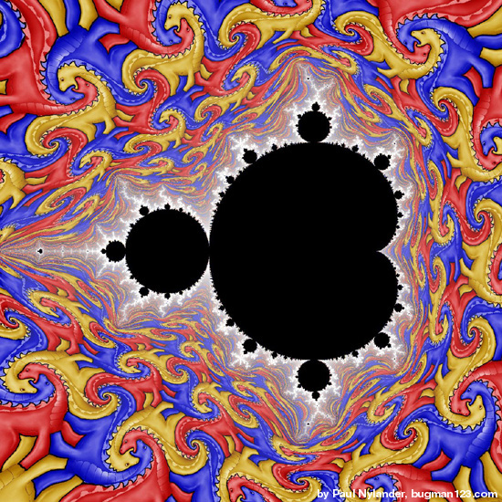
"Mandelbrot Pearls" (Mandelbrot Set Orbits), calculated in Mathematica 4.2, rendered in POV-Ray 3.6.1, 12/24/09
 The Mandelbrot set was discovered in 1980 by Beno�t Mandelbrot and is the most famous of all fractals. It is defined by iterating the function f(z) = z2 + c. For example, the third level Mandelbrot polynomial is given by F3(z) = f(f(f(z))). The Mandelbrot set is usually visualized using the Escape Time Algorithm (ETA) but another unique way to visualize this fractal is by its orbits, which are shaped like a bunch of circles and cardioids. The nth cycle orbits are the regions of c values where |Fn'(zo)| < 1 and zo is any root of Fn(zo) = zo (an attractive fixed point). The following Mathematica code was adapted from Mark McClure's Mathematica notebook:
(* runtime: 2.7 seconds *) F[z0_] := Nest[#^2 + c &, z0, n]; ToPt[z_] := {Re[z], Im[z]}; used = {}; Show[Graphics[Table[roots = Select[c /. NSolve[F[0] == 0, c], ! MemberQ[Chop[used - #], 0] &]; used = Join[used,roots]; {Hue[n/5], Map[Polygon[Table[ToPt[c /. FindRoot[{F[z] == z, D[F[z], z] == Exp[I theta]}, {c, #}, {z, #}]], {theta, 0, 2Pi, Pi/18}]] &, roots]}, {n, 1, 5}], AspectRatio -> Automatic]] Links Mathematica notebook - by Mark McClure Mandelbrot Components, Period of Hyperbolic Components - Wikipedia articles Mandelbrot Orbital Boundaries - by Donald Cross Introduction to the Mandelbrot Set - by I�igo Quilez |

 If only we could find some way to spread these pearls around in 3D, then perhaps we could create the elusive and long sought after "true 3D Mandelbrot set". A simple rotation around the x-axis looks kind of pretty, but it's certainly no true 3D Mandelbrot set. Instead, we need to find a way to rotate the pearls around their parent pearls with multiple branching and variable sizes. See also my 3D Mandelbulb orbit.
 |
Magnetic Pendulum Strange Attractor
Mathematica 4.2 version: 1/24/05; C++ version: 10/27/07; 3D rendered in POV-Ray 3.1

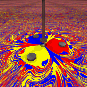

 This chaotic strange attractor represents the final resting positions for a magnetic pendulum suspended over some magnets (shown as black dots). It kind of looks like mixed paint. The 2D animation shows what happens as you decrease the damping factor. The 3D animation was shaded by path length. Click here to see an "outrageous" picture of the far field. Here is some Mathematica code:
(* runtime: 25 seconds, increase n for higher resolution *) n = 40; h = 0.25; g = 0.2; mu = 0.07; zlist = {Sqrt[3] + I, -Sqrt[3] + I, -2I}; image = Table[z2 = z[25] /. NDSolve[{z''[t] == Plus @@ ((zlist - z[t])/(h^2 + Abs[zlist - z[t]]^2)^1.5) - g z[t] - mu z'[t], z[0] == x + I y, z'[0] == 0}, z, {t, 0, 25}, MaxSteps -> 200000][[1]]; r = Abs[z2 - zlist]; i = Position[r, Min[r]][[1, 1]]; Hue[i/3], {y, -5.0, 5.0, 10.0/n}, {x, -5.0,5.0, 10.0/n}]; Show[Graphics[RasterArray[image]], AspectRatio -> 1] |
 Here is some Mathematica code to numerically solve this using the Beeman integration scheme with the predictor-corrector modification:
(* runtime: 45 seconds, increase n for higher resolution *) n = 40; tmax = 25; dt = 0.1; h = 0.25; g = 0.2; mu = 0.07; zlist = {Sqrt[3] + I, -Sqrt[3] + I, -2I}; image = Table[z = x + I y; v = a = a1 = 0; Do[z += v dt + (4a - a1)dt^2/6; vpredict = v + (3a - a1)dt/2; a2 = Plus @@ ((zlist - z)/(h^2 + Abs[zlist - z]^2)^1.5) - g z - mu vpredict; v += (2a2 + 5a - a1)dt/6; a1 =a; a = a2, {t, 0, tmax, dt}]; r = Abs[z - zlist]; Hue[Position[r, Min[r]][[1, 1]]/3], {y, -5.0, 5.0, 10.0/n}, {x, -5.0, 5.0, 10.0/n}]; Show[Graphics[RasterArray[image]], AspectRatio -> 1] The picture on the left shows another version with five magnets. See also my linked pendulum and spherical pendulum. Links Magnetic Pendulum - C++ program by Ingo Berg, uses Beeman integration scheme, here is a nice big picture and here is an animation YouTube Video - explains magnetic pendulum simulation Butterfly Effect - systems that are highly sensitive to initial conditions homemade magnetic pendulum - by David Williamson |
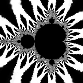
Mandelbrot Set, using Escape Time Algorithm (ETA) - original version: Java, 5/24/01; animated version: C++, 2/16/05
 zn+1 = zn2+c
This Mandelbrot set zoom animation was created using the popular Escape Time Algorithm (ETA). The animation zooms through 15 orders of magnitude. Double precision numbers are inadequate for such high resolutions, so I had to use “double-double” precision numbers, adapted from Keith Brigg’s code for double-doubles. See also my Java program and C program. Click here for some AutoLisp code. Here is some Mathematica code for this fractal: (* runtime: 1 minute *) Mandelbrot[c_] := Module[{z = 0, i = 0}, While[i < 100 && Abs[z] < 2, z = z^2 + c; i++]; i]; DensityPlot[Mandelbrot[xc + I yc], {xc, -2, 1}, {yc, -1.5, 1.5}, PlotPoints -> 275, Mesh -> False, Frame -> False, ColorFunction -> (If[# != 1, Hue[#], Hue[0, 0, 0]] &)] POV-Ray has a built-in function for this fractal: // runtime: 0.5 second camera{orthographic location <-0.5,0,-1.5> look_at <-0.5,0,0> angle 90} plane{z,0 pigment{mandel 100 color_map{[0 rgb 0][1/6 rgb <1,0,1>][1/3 rgb 1][1 rgb 1][1 rgb 0]}} finish{ambient 1}} It is also possible to render this in POV-Ray with user-defined recursive functions: // runtime: 23 seconds camera{orthographic location <-0.5,0,-1.5> look_at <-0.5,0,0> angle 90} #declare f=function(i,x,y,xc,yc) {select(i>0 & x*x+y*y<4,0,i,f(i-1,x*x-y*y+xc,2*x*y+yc,xc,yc))}; plane{z,0 pigment{function{f(100,0,0,x,y)/100}} finish{ambient 1}} Links Deep-zooming - Fractint can zoom in by magnification factors of up to 101600 Mandelbrot Deep Zoom - zooming animation, (1095) Boundary Tracing Algorithm - very fast Java applet, by John Bailey Mandelbrot & Julia Set Java Applet - interesting applet for exploring the relationship between the Mandelbrot & Julia Set, by Mark McClure |
Nebulabrot - Mathematica 4.2, 8/3/04; C++ version: 5/16/07
 This beautiful variation of the Mandelbrot set kind of resembles a nebula or a hologram. The Nebulabrot is a variation of the Buddhabrot technique. The coloring method that I used here was adapted from Paul Bourke’s web site. See also my 3D Nebulabrots. Here is some Mathematica code:
(* runtime: 10 minutes *) Mandelbrot[c_] := Length[NestWhileList[#^2 + c &, 0, Abs[#] < 2 &, 1, 1000]]; n = 275; image = Table[0, {n}, {n}]; Do[If[Mandelbrot[xc + I yc] < 1000, Module[{z = 0, iter = 0}, While[Abs[z] < 2, z = z^2 + xc + I yc; {i, j} = Floor[n{Im[z] + 1.5, Re[z] + 2}/3]; If[0 < i <= n && 0 < j <= n, image[[i, j]] += xc + I yc]; iter++]]], {xc, -2.0, 1.0, 0.01}, {yc, -1.5, 1.5, 0.01}]; Hue2[hue_, x_] := Hue[hue, Min[1, 2(1 - x)], Min[1, 2x]]; Show[Graphics[RasterArray[Map[Hue2[Arg[#]/Pi, Min[Abs[#]/18, 1]] &, image, {2}]], AspectRatio -> 1]] Links Buddhabrot animation - by Albert Lobo Buddhabrot Fractal Morphing - animation by Krzysztof Marczak Buddhabrot Cycle - animation |
Polynomial Roots - Mathematica 4.2, 12/29/08
 Strange fractal patterns emerge when you plot the complex roots of high order polynomials. This picture shows all the roots for all possible combinations of 18th order polynomials with coefficients of ±1. Notice that some parts bear a remarkable resemblance to the Heighway Dragon Curve. You can easily find the roots using Mathematica's Root function:
(* runtime: 34 seconds *) order = 12; n = 275; image = Table[0.0, {n}, {n}]; Do[Do[z = N[Root[Sum[(2Mod[Floor[(t - 1)/2^i], 2] - 1) #^(order - i), {i, 0, order}], root]]; {j,i} = Round[n({Re[z], Im[z]}/1.5 + 1)/2]; If[0 < i <= n && 0 < j <= n, image[[i, j]]++], {root, 1, order}], {t, 1, 2^order}]; ListDensityPlot[image, Mesh -> False, Frame -> False, PlotRange -> {0, 4}] You can also find all the complex roots of any high order polynomial using the Durand-Kerner method: (* runtime: 0.1 second *) n = 18; coefficients = Table[1.0, {n + 1}]; f[z_] := Sum[coefficients[[i + 1]]z^i, {i, 0, n}]; z = Table[(0.4 + 0.9I)^i, {i, 0, n - 1}]; z0 = 0.0z; While[z != z0, z0 = z; z -= f[z]/Table[Product[If[i != j, z[[i]] - z[[j]], 1], {j, 1, n}], {i, 1, n}]]; Chop[z] Chop[f[z]] Links Constrained Coefficients - beautiful plots by Loki J�rgenson description - by John Baez Integer Coefficients - slightly different plots by Dan Christensen |
2D Tree Fractal - POV-Ray version: 8/20/10, Mathematica version: 10/17/04

 This is an example of a bracketed Lindenmayer System (L-System). This technique can also be used to make lightning bolts. Here is some Mathematica code for a 2D fractal tree:
(* runtime: 0.4 second *) Tree[p1_, theta_, r_, i_] := Module[{p2 = p1 + r{Cos[theta], Sin[theta]}, graphics},graphics = {Thickness[0.07r], RGBColor[0.5r, 1 - r, 0], Line[{p1, p2}]}; If[i > 1, graphics = Join[graphics, {Tree[p2, theta - Pi/6, 0.8r, i - 1], Tree[p2, theta + Pi/4, 0.7r, i - 1]}]]; graphics]; Show[Graphics[Tree[{0, 0}, Pi/2,1, 12], AspectRatio -> 1, Background -> RGBColor[0, 0, 0], PlotRange -> {{-3, 3}, {0, 6}}]] Links Mathematica code - by Renan Cabrera |
3D Tree Fractal - POV-Ray 3.6.1, 8/20/10
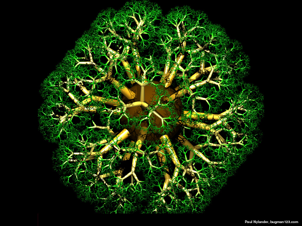
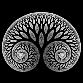
 Here are some 3D tree fractals tiled around an icosahedron. Here is some Mathematica code for a 3D fractal tree:
(* runtime: 0.7 second *) Norm[x_] := x.x; Ry[phi_] := {{Cos[phi], 0, Sin[phi]}, {0,1, 0}, {-Sin[phi], 0, Cos[phi]}}; Rz[theta_] := {{Cos[theta], -Sin[theta], 0}, {Sin[theta], Cos[theta], 0}, {0, 0, 1}}; Tree[p1_, R_, i_] := Module[{p2 = p1 + R.{0, 0, 1}, r, graphics}, r = Sqrt[Norm[p2 - p1]]; graphics = {Thickness[0.07r], RGBColor[0.5r, 1 - r, 0], Line[{p1, p2}]}; If[i > 1, graphics = Join[graphics, Table[Tree[p2, 0.6R.Rz[theta].Ry[-Pi/4], i - 1], {theta, 0, 4 Pi/3, 2Pi/3}]]]; graphics]; Show[Graphics3D[Tree[{0, 0, 0}, IdentityMatrix[3], 8]]] Here is some POV-Ray code for a 3D fractal tree: // runtime: 1 second camera{location<2,2,2> look_at <0,0,1> sky z} light_source{<2,2,2>,1} #macro tree(i) union{cone{<0,0,0>,0.1,<0,0,1>,0.06 pigment{rgb 1}} #if(i>0) union{#local j=0; #while(j<3) object{tree(i-1) rotate <0,45,0> rotate <0,0,120*j>} #local j=j+1; #end scale 0.6 translate <0,0,1>} #end} #end tree(6) Links 3D Tree Fractals - POV-Ray source code by Oliver Knill Turtle Fractals - C#.NET code to create 3D trees fractals in AutoCAD, by Kean Walmsley Tree Macros - more POV-Ray source code |
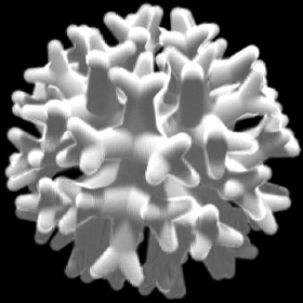
Volumetric 3D Tree Fractal - C++, C# 2005 Express Edition, 8/20/10

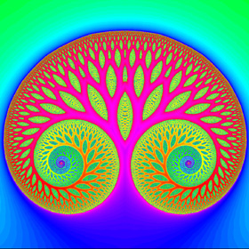
 These cloud-like 3D tree fractals were rendered using a volumetric technique similar to this technique described by Krzysztof Marczak. The images were precomputed using volumes of 175 million voxels.
 |

|
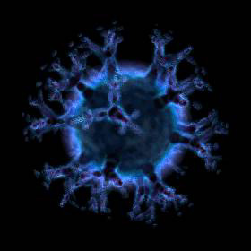
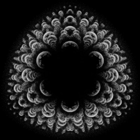
Diffusion Limited Aggregation (DLA) Fractal - Mathematica 4.2, 8/12/04; C++ version: 2/10/05
 This fractal simulates a diffusive growth process similar to that often found in nature. It is generated by single points that randomly drift around until they find something to stick to. The title on this page was generated using this technique. Here is some Mathematica code:
(* runtime: 33 seconds *) n = 100; x = y = n/2; SeedRandom[0]; image = Table[0, {n}, {n}]; Do[{x, y} = Floor[n(0.5 + 0.1{Cos[theta], Sin[theta]})] + 1; image[[x, y]] = 1, {theta, 0, 2 Pi, Pi/180}]; Do[theta = 2 Pi Random[]; {x, y} = Floor[n(1 + {Cos[theta], Sin[theta]})/2]; drift = True; While[drift, {x, y} = Mod[{x + Random[Integer, {-1, 1}], y + Random[Integer, {-1, 1}]}, n]; drift = Plus @@ Flatten[image[[Mod[x + {-1,0, 1}, n] + 1, Mod[y + {-1, 0, 1}, n] + 1]]] == 0]; image[[x + 1, y + 1]] = 1 - t/360, {t, 0, 360}]; ListDensityPlot[image, Mesh -> False, Frame -> False] |
 Links
LinksAndy Lomas - impressive 3D aggregation simulations rendered with ambient occlusion Lichtenberg Figures - beautiful electric discharge patterns 3D DLA Cluster - by Chris Rycroft 3D DLA - by Mark Stock 3D DLA Fractals - by Paul Bourke Java Applet - by Chi-Hang Lam Dielectric Breakdown Model - simulates lightning bolts Snowflake Simulations - rendered in POV-Ray, by Theodore Kim and Ming Lin SnowFlake Cellular Automata - by Ramiro Perez Snowfake Movies - cellular automata Snow Crystals - Cal Tech’s beautiful guide to snowflakes, be sure to see the growing snowflake movie giant snowflake - from an Alaskan permafrost tunnel Frost Flowers - very weird ice that looks like hair simple Snowflake algorithm - by Clifford Reiter rapid crystal growth - as part of the National Ignition Facility Project Century Egg - unusual Chinese delicacy that can have dendrite-like patterns growing on it |
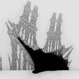
Weierstrass Function, POV-Ray 3.6.1: 5/18/08, Mathematica 4.2: 3/2004
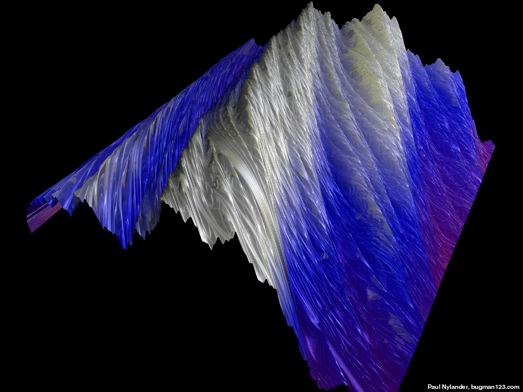
 The infamous Weierstrass function is an example of a function that is continuous but completely undifferentiable. Here is some Mathematica code: (* runtime: 0.7 second *) Plot3D[Sum[Sin[Pi k^a x]/(Pi k^a), {k, 1, 50}], {x, 0, 1}, {a, 2, 3}, PlotPoints -> 100] |
Romanesco Broccoli, 2/29/12
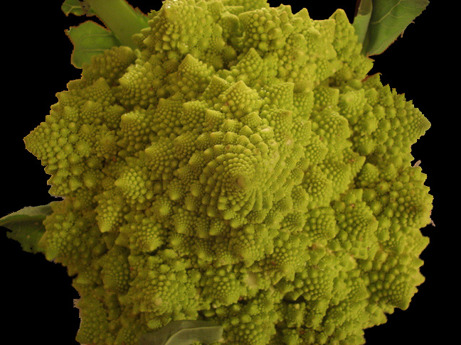 Here is a Romanesco Broccoli, famous for it fractal-like structure. My wife found these at a local farm and bought one as a gift for me. They taste great!
 |
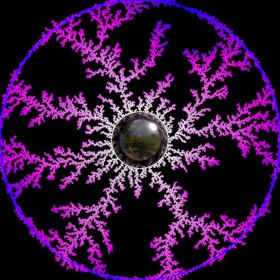
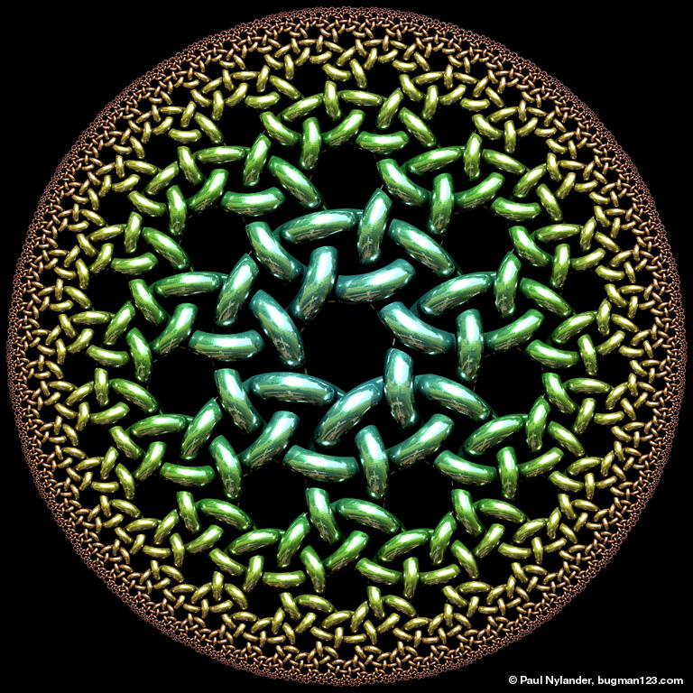
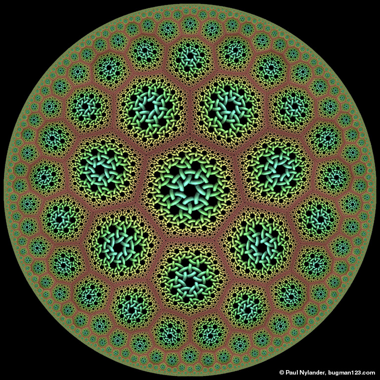
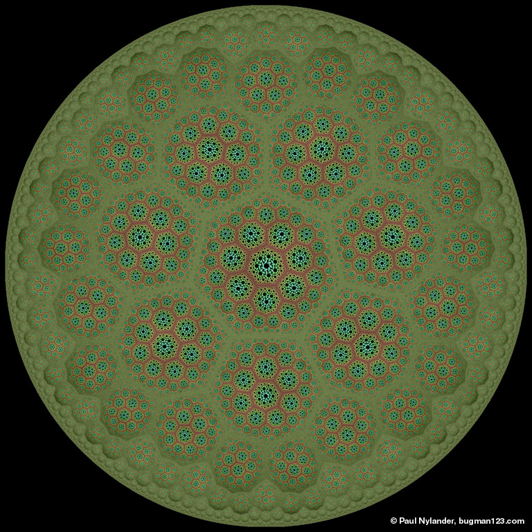
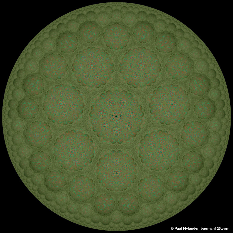
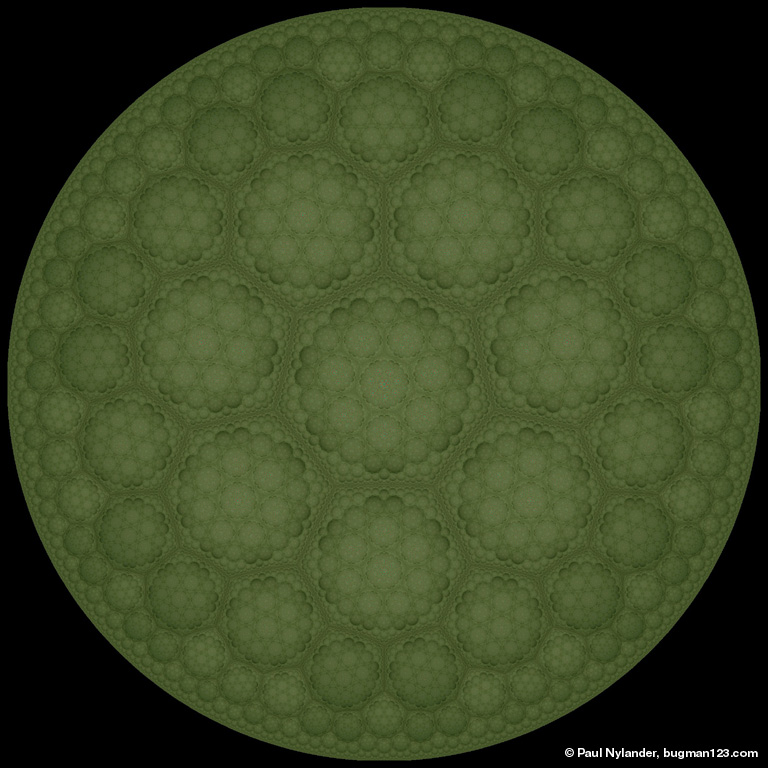
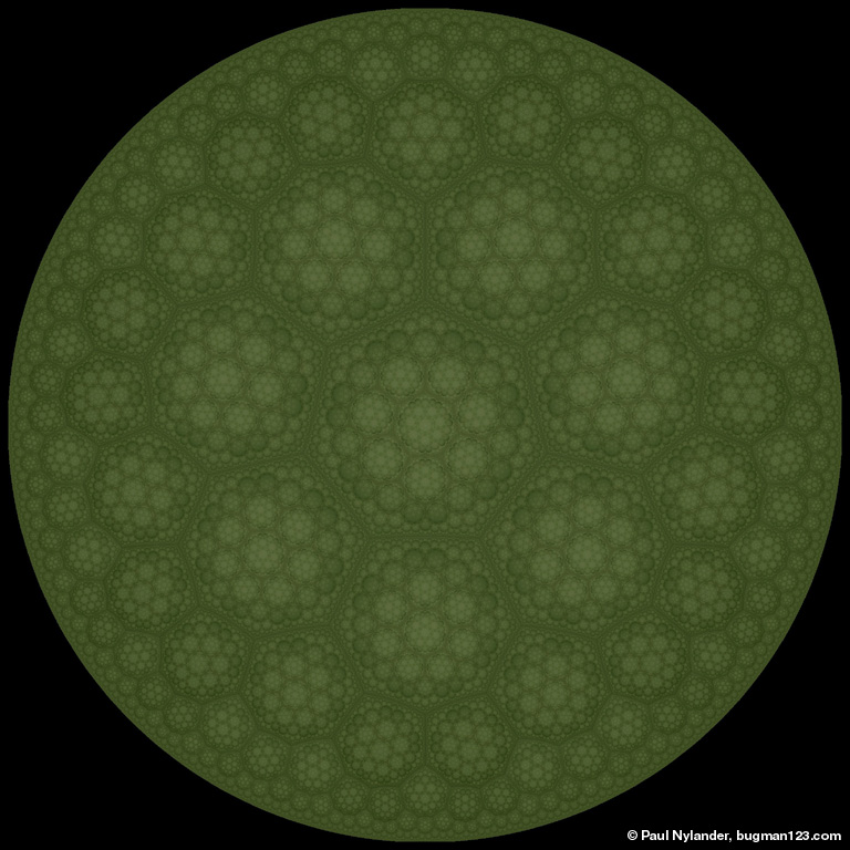
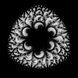
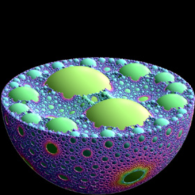
Recursive (7,3) Poincaré Hyperbolic Disk - AutoLisp, POV-Ray 3.6.1, C#, 5/17/11
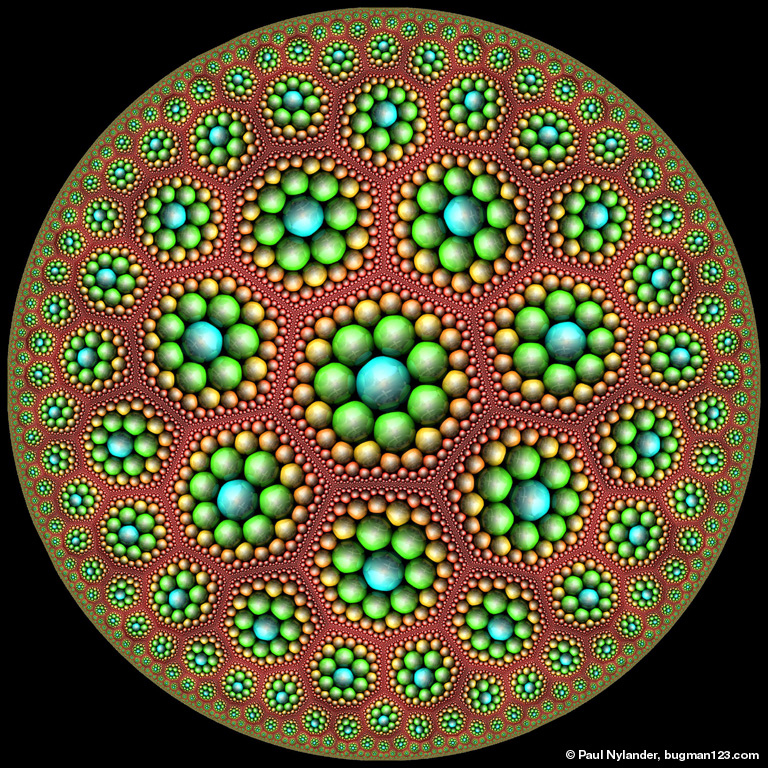 Here is a circular Poincaré disk composed of smaller Poincaré disks shaped like hyperbolic polygons. The small disks were shaped into hyperbolic polygons using a conformal mapping technique. See also my other conformal mappings of the Poincaré disk.
 |
Links Sporogenesis, Blooming - beautiful recursive Poincaré tessellations, by Zueuk |
Wada Basin - Mathematica 4.2, 6/19/05; C++ version: 9/11/08

 To make a Wada basin, simply put some Christmas tree ornaments together. The following Mathematica code demonstrates how to write a very simple ray tracer. Click here to download a simple C++ program.
(* runtime: 65 seconds, increase n for higher resolution *) n = 140; r = 1; plight = {0, 0, 1}; Normalize[x_] := x/Sqrt[x.x]; spheres = {{{1, 1.0/Sqrt[3], 0}, {1, 0,0}}, {{-1, 1.0/Sqrt[3], 0}, {0, 1, 0}}, {{0, -2.0/Sqrt[3], 0}, {0, 0, 1}}, {{0, 0, -Sqrt[8.0/3]}, {1, 1, 1}}}; Intersections[p_, dir_] := Module[{a = p.dir, b}, b = r^2 + a^2 - p.p; If[b > 0, Select[Sqrt[b]{-1, 1} - a, # > 10^-10 &], {}]]; RayTrace[p_, dir_, depth_] := Module[{dlist = Map[Min[Intersections[p - #[[1]], dir]] &, spheres], d, i, p2, normal, color, lightdir, intensity}, d = Min[dlist]; If[d < Infinity, p2 = p + d dir; i = Position[dlist, d][[1, 1]]; normal = Normalize[p2 - spheres[[i, 1]]]; color = If[depth > 50, {0, 0, 0}, RayTrace[p2, Normalize[dir - 2(normal.dir)normal], depth + 1]]; lightdir = Normalize[plight - p2]; intensity = normal.lightdir; If[intensity > 0, shadowed = Or @@ Map[Intersections[p2 - #[[1]], lightdir] =!= {} &, spheres]; If[! shadowed,color += intensity spheres[[i, 2]]]]; color, {0, 0, 0}]]; Show[Graphics[RasterArray[Table[RGBColor @@ Map[Min[1, Max[0, #]] &, RayTrace[{0, 0, 1},Normalize[{x,y, -1}], 1]], {y, -0.5, 0.5, 1.0/n}, {x, -0.5, 0.5, 1.0/n}]], AspectRatio -> 1]] You can also easily ray trace Wada Basins using POV-Ray: // runtime: 4 seconds global_settings{max_trace_level 50} camera{location z look_at 0} light_source{z,1} #default{finish{reflection 1 ambient 0}} sphere{<1,sqrt(1/3),0> 1 pigment{rgb <1,0,0>}} sphere{<-1,1/sqrt(3),0> 1 pigment{rgb <0,1,0>}} sphere{<0,-2/sqrt(3),0> 1 pigment{rgb <0,0,1>}} sphere{<0,0,-sqrt(8/3)> 1 pigment{rgb 1}} Links Simplicity to Complexity - Maya article by Duncan Brinsmead Indra's Deep Sea Life - beautiful POV-Ray images by Kevin Wampler Making Fractals with Christmas Ornaments - photos by Keenan Crane Scratch a Pixel - ray-tracing tutorial with source code Javascript Ray Tracer - simple Javascript ray tracer by John Haggerty |
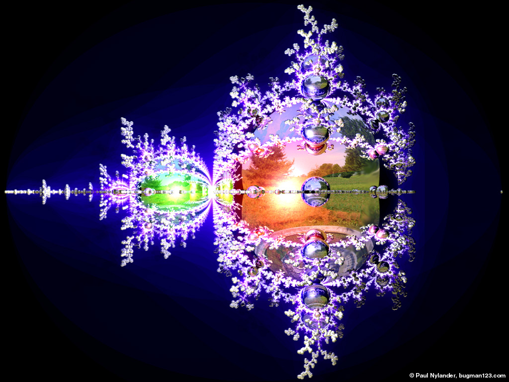
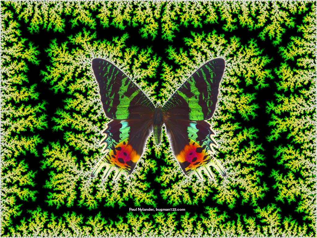
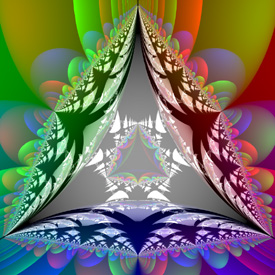
“The Watering Hole” Orbit Trap - old version: Mathematica 4.2, 2/26/05; animated version: C++, 7/12/06

 Orbit trapping is a popular technique for mapping arbitrary shapes to a fractal. This orbit trap is shaped like a Sunset Moth. See also my 3D orbit trap fractals. Here is some basic Mathematica code:
(* runtime: 18 seconds, Note: black areas of Picture.bmp will be transparent *) image = Import["C:/Picture.bmp"][[1, 1]]/255.0; i2 = Length[image]; j2 = Length[image[[1]]]; n = 275; map[z_] := Round[{i2(Im[z] + 1), j2(Re[z] + 1)}/2]; trapped[i_, j_] := 0 < i <= i2 && 0 < j <= j2 && image[[i, j]] != {0, 0, 0}; OrbitTrap[c_] := Module[{z = 0, i, j, k = 0}, While[k < 100 && Abs[z] < 2 && (k < 2 || ! trapped @@ map[z]), z = z^2 + c;k++]; {i, j} = map[z]; If[trapped[i, j], RGBColor @@ image[[i, j]], RGBColor[0, 0, 0]]]; Show[Graphics[RasterArray[Table[OrbitTrap[xc + I yc], {yc, -1.5, 1.5, 3.0/n}, {xc, -2, 1, 3.0/n}]], AspectRatio -> 1]] Links impressive orbit traps fractals - created by Tom Beddard using his Fractal Explorer plugin for Photoshop |
Gears Orbit Trap - POV-Ray 3.1, C++, 7/12/06
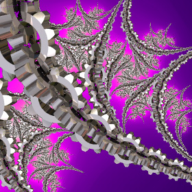
 Here is the same fractal again using a gear-shaped orbit trap.
 |
Mandelbrot Set Tessellation - Mathematica 4.2, 6/14/04
 The left image is distorted because it is not a hyperbolic tiling. For more information, see Bill Rood’s web site and the book “The Colours of Infinity”. Here is some basic Mathematica code:
(* runtime: 70 seconds *) image = Import["C:/Picture.jpg"][[1, 1]]; n = Length[image]; m = Length[image[[1]]]; Show[Graphics[RasterArray[Table[Module[{c = x + I y, z = 0.0}, Do[z = z^2 + c, {25}]; RGBColor @@ (image[[Floor[n Mod[Re[Log[Log[z]]]m/n, 1]] + 1, Floor[m Mod[2Arg[c], 1]] + 1]]/255.0)], {y, -1.5, 1.5, 3/275}, {x, -2, 1, 3.0/275}]], AspectRatio -> 1]] |
Golden Ratio Spiral Orbit Trap - Mathematica 4.2, 3/3/05

 Here is an orbit trap in the shape of the Golden Ratio Spiral. Here is some Mathematica code:
(* runtime: 1 minute *) phi = 0.5(1 + Sqrt[5]); f[z_] := Module[{r = Log[Abs[z]]/(4Log[phi]) - Arg[z]/(2Pi)}, 18Abs[r - Round[r]]]; OrbitTrap[c_] := Module[{z = 0, i =0}, While[i < 100 && Abs[z] < 100 && (i < 2 || f[z] > 1), z = z^2 + c; i++]; Hue[Arg[z]/(2Pi), Min[1, 2 f[z]], Max[0, Min[1, 2(1 - f[z])]]]]; Show[Graphics[RasterArray[Table[OrbitTrap[xc + I yc], {yc, -1.5, 1.5, 3.0/275}, {xc, -2, 1, 3.0/275}]], AspectRatio -> 1]] |
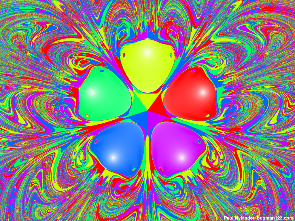
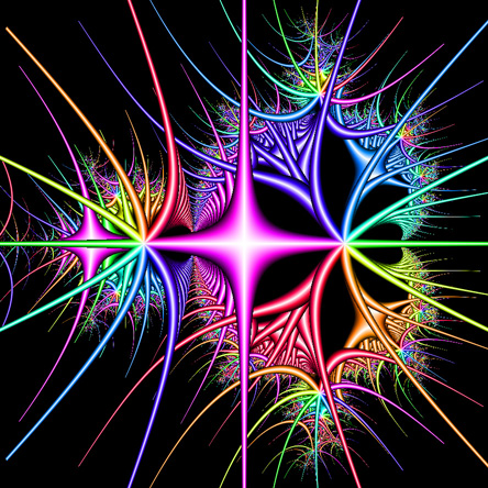
Newton-Raphson Fractal - Mathematica 4.2, 6/17/04
 f(z) = z5-1, zn+1 = zn - f(zn)/f'(zn)
It is surprisingly easy to make these beautiful fractals. Here is some Mathematica code: (* runtime: 25 seconds *) f[z_] := z^5 - 1; Show[Graphics[RasterArray[Table[data = FixedPointList[# - f[#]/f'[#] &, x + I y, 29]; z = 1 - Length[data]/30; Hue[Arg[Last[data]]/(2Pi), Min[1,2(1 - z)], Min[1, 2z]], {y, -1.5, 1.5, 3.0/275}, {x, -1.5, 1.5, 3.0/275}]]], AspectRatio -> 1] Links Newton-Raphson Fractal - Mathematica code by Mark McClure Newton-Raphson Fractal - Mathematica code by Robert M. Dickau |
Julia Set Fractal - Mathematica 4.2: 4/15/04, POV-Ray 3.6.1: 7/4/06
 zn+1 = zn2+c, c = -0.63-0.407i
Julia sets were discovered by Gaston Maurice Julia. Here is some Mathematica code: (* runtime: 17 seconds *) Julia[z0_] := Module[{z = z0, i = 0}, While[i < 100 && Abs[z] < 2, z = z^2 + c; i++]; i]; c = -0.63 - 0.407 I; DensityPlot[Sqrt[Julia[x + I y]], {x, -1.5, 1.5}, {y, -1.5, 1.5}, PlotPoints -> 275, Mesh -> False, Frame -> False, ColorFunction -> Hue] POV-Ray has a built-in function for these fractals: // runtime: 0.5 second camera{orthographic location <0,0,-1.5> look_at 0 angle 90} plane{z,0 pigment{julia <-0.63,-0.407>,200} finish{ambient 1}} |
Cubic Julia Set Fractal - original version: Java, 6/9/01; animated version: Mathematica 4.2, 2/18/05

 zn+1 = zn3+c, c = -0.5-0.05i
This was one of my older favorites. Here is some Mathematica code demonstrating a simple technique called the Escape Time Algorithm (ETA): (* runtime: 11 seconds *) c = -0.5 - 0.05 I; Julia[z0_] := Module[{z = z0, i = 0}, While[i < 100 && Abs[z] < 2, z = z^3 + c; i++]; i]; DensityPlot[Julia[x + I y], {x, -1.15, 1.15}, {y, -1.15, 1.15}, PlotPoints -> 275, Mesh -> False, Frame -> False, ColorFunction -> (RGBColor[Min[2#^2, 1], Max[2# - 1, 0], Min[2#, 1]] &)] This is how you can make this fractal in POV-Ray: // runtime: 0.5 second camera{orthographic location <0,0,-1.15> look_at 0 angle 90} plane{z,0 pigment{julia <-0.5,-0.05>,30 exponent 3 color_map{[0 rgb 0][1/3 rgb <0,0,1>][2/3 rgb <1,0,1>][1 rgb 1]}} finish{ambient 1}} |
Distance Estimation - Mathematica 4.2, 11/1/09

 Here is some Mathematica code demonstrating how to find a distance of any point outside the Mandelbrot set that is "guaranteed" not to reach any point inside the Mandelbrot set. Note that the actual distance to the Mandelbrot set should always be somewhat larger than this distance. But be advised that I am not entirely sure if this code is correct. The nice thing about this approach is that it emphasizes the fine details near the boundary better than the Escape Time Algorithm (ETA). It is also useful for efficiently ray tracing 3D hypercomplex fractals:
(* runtime: 36 seconds *) DistanceEstimate[c_] := Module[{z = 0, dz = 1, i = 0, loop = True, r}, While[loop, z = z^2 + c; r = Abs[z]; i++;loop = (i < 100 && r < 2); If[loop, dz *= 2z]]; 0.5r Log[r]/Abs[dz]]; DensityPlot[DistanceEstimate[xc + I yc], {xc, -2.3, 0.7}, {yc, -1.5, 1.5}, PlotPoints -> 275, Mesh -> False, Frame -> False, PlotRange -> {0, 0.001}] |
 Here is some Mathematica code for distance estimation of a cubic Julia set:
(* runtime: 15 seconds *) c = -0.5 - 0.05I; DistanceEstimate[z0_] := Module[{z = z0, dz = 0, i = 0, r = 1}, While[i < 100 && r <2, dz = 3z^2 dz + 1; z = z^3 + c; r = Abs[z]; i++]; 0.5r Log[r]/Abs[dz]]; DensityPlot[DistanceEstimate[x + I y], {x, -1.15, 1.15}, {y, -1.15, 1.15}, PlotPoints -> 275, Mesh ->False, Frame -> False, PlotRange -> {0, 0.001}] Links Distance Rendering for Fractals - article by I�igo Quilez |
Inverse Julia Set Fractal - Mathematica 4.2, 6/26/04
 The following Mathematica code demonstrates how to create a Julia set using the Inverse Iteration Method (IIM). This technique is good for showing the edges of the set, but some regions are faint because they attract much slower:
(* runtime: 4 seconds *) c = -0.5 - 0.05 I; zlist = {0}; Do[zlist = Flatten[Map[(# - c)^(1/3){1, -(-1)^(1/3) , (-1)^(2/3)} &, zlist], 1], {10}]; ListPlot[{Re[#], Im[#]} & /@ zlist, PlotStyle -> PointSize[0.005], AspectRatio -> Automatic] There are a variety of Modified Inverse Iteration Methods (MIIM) which can be used to speed up the calculation by pruning dense branches of the tree. One such method is to prune branches when the map becomes contractive (the cumulative derivative becomes large). The following Mathematica code was adapted from Peter Liepa's source code: (* runtime: 3 seconds *) power = 3; c = -0.5 - 0.05 I; zlist = {}; imax = 100; z = Table[0, {imax}]; dz = Table[1, {imax}]; roots = Table[1, {imax}]; i = 2; While[i > 1, z[[i]] = {1, -(-1)^(1/3), (-1)^(2/3)}[[roots[[i]]]](z[[i - 1]] - c)^(1/power); dz[[i]] = power Abs[z[[i]]]^(power - 1)dz[[i - 1]]; zlist =Append[zlist, z[[i]]]; If[i < imax && dz[[i]] < 250.0, i++; roots[[i]] = 1, While[i > 1 && roots[[i]] == power, roots[[i]] = 1; i--]; roots[[i]]++]]; ListPlot[{Re[#],Im[#]} & /@ zlist, PlotStyle -> PointSize[0.005], AspectRatio -> Automatic] Here is another approach for creating MIIM Julia sets, based on pixel hit counts: (* runtime: * minutes *) Here is another approach for creating MIIM Julia sets, adapted from Mark McClure’s Mathematica code: (* runtime: 4 seconds *) InvertList[zlist_] := Flatten[Map[Floor[130(# - c)^(1/3){1, -(-1)^(1/3), (-1)^(2/3)}]/130 &, zlist], 1]; c = -0.5 - 0.05 I; zlist = Nest[InvertList, {0}, 8]; zlist2 = zlist; While[zlist2 =!= {}, zlist2 = Complement[InvertList[zlist2],zlist]; zlist = Union[zlist2, zlist]]; ListPlot[{Re[#], Im[#]} & /@ zlist,PlotStyle -> PointSize[0.005], AspectRatio -> Automatic] |
 Links
LinksSome Julia Sets - by Michael Becker, see also pages 2, 3, 4 Fractal Field Guide - by Peter Liepa Inverse Iteration Fractals - by Ramiro Perez Java Applet - by Mark McClure |
Inverse Mandelbrot Set Fractal, 12/22/09
 The Mandelbrot set is defined by iterating the function f(z) = z2 + c. For example, the third level Mandelbrot polynomial is given by F3(z) = f(f(f(z))). Now, suppose we arbitrarily choose a "seed" value of z = 0 and solve for the roots of c such that Fn(0) = 0. Here is a plot of the roots of the 21st level Mandelbrot polynomial showing a total of 1,048,576 roots (calculated courtesy of Abdelaziz Merzouk). Of course, this is still a far cry from the inverse Julia set pruning methods which can probe thousands of levels deep, but unfortunately, there is no similar way to prune Mandelbrot set roots (as far as I know). Here is some Mathematica code:
(* runtime: 30 seconds *) imax = 8; z = c /. Solve[Nest[#^2 + c &, 0.0, imax] == 0, c]; ListPlot[Map[{Re[#], Im[#]} &, z], AspectRatio -> 1] You can also find these roots using the Durand-Kerner method: (* runtime: 38 seconds *) imax = 7; order = 2^(imax - 1); F[c_] := Nest[#^2 + c &, 0.0, imax]; z = Table[(0.4 + 0.9I)^i, {i, 1, order}]; z0 = 0.0z; While[Max[Abs[z - z0]] > 1.0*^-7, z0 = z; z -= F[z]/Table[Product[If[i != j, z[[i]] - z[[j]], 1], {j, 1, order}], {i, 1, order}]]; ListPlot[Map[{Re[#], Im[#]} &, z], AspectRatio -> 1] Links Eigenvalue Iter Examples - by Steven Fortune Mandelbrot Orbits - another interesting approach, by Donald Cross Roots of the 21st level Mandelbrot polynomial (1,048,576 roots) - by Piers Lawrence |
Glynn Julia Set Fractal, Mathematica 4.2, 10/13/09
 The Glynn Set is a special Julia Set, named after Earl Glynn. It kind of looks like a tree. See also my 3D Glynn Julia set. Here is some Mathematica code:
(* runtime: 48 seconds *) Julia[z0_] := Module[{z = z0, i = 0}, While[i < 100 && Abs[z] < 2, z = z^1.5 + c; i++]; i]; c = -0.2; DensityPlot[Julia[-x + I y], {y, -0.2, 0.2}, {x, 0.35, 0.75}, PlotPoints -> 275, Mesh -> False, Frame -> False] Here is some code to plot this using the Modified Inverse Iteration Method (MIIM). Note that special care must be taken to verify each root's validity: (* runtime 7 seconds *) Pow[z_, n_, k_] := Module[{theta = Arg[z]}, theta = n(theta + 2Pi (k - Floor[(theta/Pi +Abs[1/n])/2])); If[Abs[theta] > Pi, Null, Abs[z]^n Exp[I theta]]]; power = 1.5; nroot = 3; c = -0.2; zlist = {}; dzmax = 25.0; imax =1000; z = Table[-0.61, {imax}]; dz = Table[1, {imax}]; roots = Table[1, {imax}]; i = 2; While[i > 1, z[[i]] = Pow[z[[i - 1]] - c, 1/power, roots[[i]] - 1]; If[z[[i]] === Null, prune = True, dz[[i]] = Abs[power]Abs[z[[i]]]^(power - 1)dz[[i - 1]]; zlist = Append[zlist, z[[i]]]; prune = (i == imax || dz[[i]] > dzmax)]; If[prune, While[i > 1 && roots[[i]] == nroot, roots[[i]] = 1; i--]; roots[[i]]++, i++; roots[[i]] = 1]]; ListPlot[{Re[#], Im[#]} & /@ zlist, PlotStyle -> PointSize[0.005], AspectRatio ->Automatic] |
 These ones are incorrect, but I still think they look interesting.
Links Fractal Tree discussion - on Fractal Forums FnGlynn - Youtube animation |
Burning Ship Fractal - Mathematica 4.2, 8/5/04
 zn+1 = (|xn| + i |yn|)2 - c = xn2 - yn2 + 2 i |xnyn| - c
This weird picture is a modified form of the Mandelbrot set. It’s amazing what kind of pictures you can get with the right equations. Here is some Mathematica code: (* runtime: 5 minutes *) BurningShip[c_] := Module[{x = 0, y = 0, i = 0}, While[x^2 - y^2 < 200 && i < 250, {x, y} = {x^2 - y^2, 2Abs[x y]} - c; i++]; i]; DensityPlot[-BurningShip[{xc, yc}], {xc, 1.71, 1.8}, {yc, -0.01, 0.08}, PlotPoints -> 275, Mesh -> False, Frame -> False] Links Burning Ship Fractal - by Paul Bourke Burning Bulb - 3D Burning Ship fractal based on the triplex, by Christian Kleinhuis |
Barnsley’s Fern - Mathematica 4.2, 10/16/04
 This is an example of a Directed Graph Iterated Function System (Digraph IFS). The image is generated by randomly selecting transformations which jump to different points on the fern. Here is some Mathematica code:
(* runtime: 7 seconds *) n = 275; p = {0, 0}; image = Table[0, {n}, {n}]; Do[x = Random[Integer, 99]; p = Which[x < 3, {{0, 0}, {0, 0.16}}.p,x < 76, {{0.85, 0.04}, {-0.04, 0.85}}.p + {0, 1.6}, x <89, {{0.2, -0.26}, {0.23, 0.22}}.p + {0, 1.6}, True, {{-0.15, 0.28}, {0.26, 0.24}}.p + {0, 0.44}]; image[[Floor[n(p[[1]]/10 + 0.5)] + 1, Floor[n p[[2]]/10] + 1]]++, {100000}]; Show[Graphics[RasterArray[Map[RGBColor[0, 1 - Exp[-0.1#], 0] &, image, {2}]], AspectRatio -> 1]] Links XenoDream - free software for creating 3D IFS fractals, uses holons to define the IFS fractal, uses a z-buffer as a surface for lighting, by Garth Thornton Incendia - software for creating beautiful 3D IFS fractals, by Ramiro Perez, see his gallery, be sure to see Apollonian Flowers Open Me Slowly - 3D IFS animation by Kris Northern Inside the Sierpinski Temple - 3D IFS animation, by David Makin 3D Fractal Broccoli - Romanesco Broccoli, rendered with PhotoRealistic RenderMan, by Aleksandar Rodic Romanesco Broccoli molds - by Cayetano Ramirez Video Feedback - amazing video feedback fractals by Peter King |
Flame Fractal - Mathematica 4.2, 3/5/05
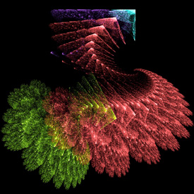 Flame Fractals are a popular, generalized variation of IFS fractals, invented by Scott Draves. This one is based on the Apophysis sample parameters. See also my POV-Ray code. Here is some Mathematica code:
(* runtime: 25 seconds *) V1[{x_, y_}] := {Sin[x], Sin[y]}; F1[p_] := Module[{p2 = {{0.81, -0.33}, {0.08, 0.89}}.p + {0.24, -0.07}}, 0.88p2 + 0.12V1[p2]]; F2[p_] := Module[{p2 = {{0.3, 0.52}, {-0.56, 0.37}}.p + {-0.09, -0.42}}, 0.88p2 + 0.12V1[p2]]; F3[p_] := V1[{{-0.43, 0.38}, {-0.2, -0.44}}.p + {1.74, 1.21}]; F4[p_] := V1[{{-0.49, -0.27}, {0.28, -0.53}}.p + {0.51, 0.62}]; w1 = 0.65; w2 = 0.29; w3 = 0.03; w4 = 0.03; n = 275; image = Table[{0, 0, 0}, {n}, {n}]; p = {0, 0}; Do[x = Random[]; k = Which[x < w1, 1, x < w1 + w2, 2, x < w1 + w2 + w3, 3, True, 4]; p = {F1, F2, F3, F4}[[k]][p]; {j,i} = Round[n{p[[1]] + 1.1, p[[2]] + 1.8}/3]; image[[i, j]] += List @@ ToColor[Hue[k/4.0], RGBColor], {100000}]; Show[Graphics[RasterArray[Map[RGBColor @@ Map[(1 - Exp[-0.2#]) &, #] &, image, {2}]], AspectRatio -> 1]] Links Flowers - a beautiful fractal bouquet, by Keith Mackay Fleur D'apo - by Mynameishalo Ice Flower - by Ulliroyal Cory Ench - some impressive flame fractals, some of my favorites are Downey and Genesis Soup Apophysis - free Flame Fractal software Flame Fractal Java applet |
Clifford Attractor - adapted from Paul Richards, Mathematica 4.2, 12/27/04
 xn+1 = sin(a yn) + c cos(a xn)
yn+1 = sin(b xn) + d cos(b yn) This type of strange attractor was invented by Clifford Pickover. If you look closely, you may find what appears to be distorted bifurcation fractals in the image. The right image is a superposition of many Clifford Attractors. See also my POV-Ray code. Here is some Mathematica code: (* runtime: 3 minutes *) n = 275; image = Table[{0, 0, 0}, {n}, {n}]; Interpolate[p_, x1_, x2_] := 2Cos[ArcCos[x1/2] + p(ArcCos[x2/2] - ArcCos[x1/2])]; Do[a = Interpolate[p,1.6, 1.3]; b = Interpolate[p, -0.6, 1.7]; c = Interpolate[p, -1.2, 0.5]; d = Interpolate[p, 1.6, 1.4]; x = y = 0; Do[{x, y} = {Sin[a y] + c Cos[a x], Sin[b x] + d Cos[b y]}; {i, j} = Round[n({y, x}/6 + 0.5)]; If[0 < i <= n && 0 < j <= n,image[[i, j]] += List @@ ToColor[Hue[p], RGBColor]], {1000}], {p, 0, 1, 0.001}]; Show[Graphics[RasterArray[Map[RGBColor @@ Map[1 - Exp[-0.02#] &, List @@ #] &, image, {2}]], AspectRatio -> 1]] Links Polynomial - game by Dmytry Lavrov |
Frequency Filtered Random Noise - Mathematica 4.2, 9/5/04
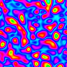
 This technique uses a Fourier transform to generate random periodic textures. See also my image deconvolution. Here is some Mathematica code:
(* runtime: 20 seconds *) n = 275; SeedRandom[1]; ListDensityPlot[Abs[InverseFourier[Fourier[Table[Random[], {n}, {n}]] Table[Exp[-((j/n - 0.5)^2 + (i/n - 0.5)^2)/0.025^2], {i, 1, n}, {j, 1, n}]]], Mesh -> False, Frame -> False, ColorFunction -> (Hue[# + 0.5] &)] Here is some Mathematica code for an animated version. This technique can be used for simulating water surfaces: (* runtime: 18 seconds *) n = 64; SeedRandom[0]; Scan[ListDensityPlot[#, Mesh -> False, Frame -> False, ColorFunction -> (Hue[# + 0.5] &)] &, Abs[InverseFourier[Fourier[Table[Random[], {32}, {n}, {n}]]Table[Exp[-((i/n - 0.5)^2 + (j/n - 0.5)^2 + (t/32 - 0.5)^2)/0.025^2], {t, 1, 32}, {i, 1, n}, {j, 1, n}]]]] |
Perlin Noise - Mathematica 4.2, 8/16/04
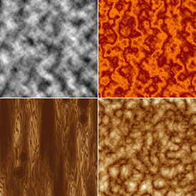 This is a popular technique for generating all kinds of random periodic textures such as artificial terrain, clouds, water, wood, fire, marble, etc.. It was invented by Ken Perlin. Most random number generators base subsequent random numbers on their previous numbers. In this way, highly complicated “random” scenes can be easily reconstructed from a single initial seed number. Here is some Mathematica code:
(* runtime: 2 minutes *) Interpolate[{y0_, y1_, y2_, y3_}, mu_] := (y3 - y2 - y0 + y1)mu^3 + (2 y0 - 2 y1 + y2 - y3) mu^2 + (y2 - y0) mu + y1; m = 14; SeedRandom[0]; noise = Table[Random[], {m}, {m}]; Noise[x0_, y0_] := Module[{x = Mod[x0, 1], y = Mod[y0, 1], i0, j0}, i0 = Floor[m y]; j0 = Floor[m x]; Interpolate[Table[Interpolate[Table[noise[[Mod[i, m] + 1, Mod[j, m] + 1]], {j, j0 - 1, j0 + 2}], m x - j0], {i, i0 - 1, i0 + 2}], m y - i0]]; a = 2; b = 2; n = 275; image = Table[Sum[Noise[b^i x, b^i y]/a^i, {i, 0, 4}], {x, 0.0, 1.0, 1.0/n}, {y, 0.0, 1.0, 1.0/n}]; ListDensityPlot[image, Mesh -> False, Frame -> False] Here is some Mathematica code that uses a triangle wave to make Perlin noise that looks like marble: (* runtime: 4 seconds *) ListDensityPlot[Table[t = 5j/n +image[[i, j]]; Mod[t, 1] - 2Mod[t + 0.5, 1]Floor[Mod[t, 1] + 0.5], {i, 1, n}, {j, 1, n}], Mesh -> False, Frame -> False, ColorFunction -> (RGBColor[1 - 0.5#, 0.5(1 - #), 0] &)] Here is some Mathematica code to make it look like granite: (* runtime: 2 minutes *) ListDensityPlot[Table[f = 2^i; Sum[Abs[0.5 - Noise[f x, f y]]/f, {i, 0, 5}], {x, 0.0, 1.0, 1.0/n}, {y, 0.0, 1.0, 1.0/n}], Mesh -> False, Frame -> False] |
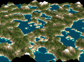 Here is some Mathematica code to plot the Perlin noise as an artificial terrain (you must run the above Perlin noise code before you can run this code):
(* runtime: 10 seconds *) Gradient2[x_, grad_] := Module[{i = 1, n = Length[grad]}, While[i <= n && grad[[i, 1]] < x, i++]; RGBColor @@ If[1 < i <= n, Module[{x1 = grad[[i - 1, 1]], x2 = grad[[i, 1]]}, ((x2 - x) grad[[i - 1, 2]] + (x - x1)grad[[i, 2]])/(x2 - x1)], grad[[Min[i, n], 2]]]]; EarthTones = {{0, {0, 0.1, 0.24}}, {0.1, {0, 0.6, 0.6}}, {0.1, {0.9, 0.8, 0.6}}, {0.2, {0.5, 0.4, 0.3}}, {0.5, {0.2, 0.3, 0.1}}, {0.8, {0.7, 0.6, 0.4}}, {0.8, {1, 1, 1}}, {1, {1, 1, 1}}}; Show[SurfaceGraphics[Map[Max[#, 1] &, image, {2}], Mesh -> False, Boxed -> False, BoxRatios -> {1, 1, 1/12}, ColorFunction -> (Gradient2[1.3#, EarthTones] &), Background -> RGBColor[0, 0, 0]]] See also my Terragen terrain. |
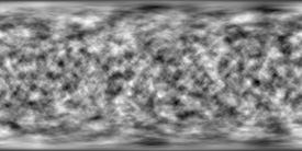 Here is some Mathematica code to map Perlin noise to a sphere as described on Paul Bourke’s web site. This is accomplished by evaluating a 3D Perlin noise “cloud” at points on the sphere:
(* runtime: 7 minutes *) m = 14; SeedRandom[0]; noise = Table[Random[], {m}, {m}, {m}]; Noise[x0_, y0_, z0_] := Module[{x = Mod[x0, 1], y = Mod[y0, 1], z = Mod[z0, 1], i0, j0, k0}, i0 = Floor[m y]; j0 = Floor[m x]; k0 = Floor[m z]; Interpolate[Table[Interpolate[Table[Interpolate[Table[noise[[Mod[i, m] + 1, Mod[j, m] + 1, Mod[k, m] + 1]], {j, j0 - 1, j0 + 2}], m x - j0], {i, i0 - 1, i0 + 2}], m y - i0], {k, k0 - 1, k0 + 2}], m z - k0]]; a = 2; b = 2; Perlin[x_, y_, z_] := Sum[Noise[b^i x, b^i y, b^i z]/a^i, {i, 0, 4}]; image = Table[Perlin[Cos[theta]Sin[phi], Sin[theta]Sin[phi], Cos[phi]], {phi, 0, Pi, Pi/180}, {theta, 0, 2Pi, Pi/180}]; ListDensityPlot[image, Mesh -> False, Frame -> False, AspectRatio -> Automatic, ImageSize -> {360, 180}] |
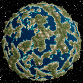 Here is some Mathematica code to plot Perlin noise as an artificial planet (you must run the above Perlin noise code before you can run this code):
(* runtime: 7 minutes *) ParametricPlot3D[Module[{x = Cos[theta]Sin[phi], y = Sin[theta]Sin[phi], z = Cos[phi], w}, w = Max[0, Perlin[x, y, z] - 0.8]; Append[(1 + 0.1w){x, y, z}, {EdgeForm[], Gradient2[w, EarthTones]}]], {theta, 0, Pi}, {phi, 0, Pi}, PlotPoints -> {361, 181}, Background -> RGBColor[0, 0, 0], Boxed -> False, Axes -> None, Lighting -> False]  This animated sun effect was generated by translating the noise over time. Here is some sample POV-Ray code:
// runtime: 0 second camera{location <0,0,2.25> look_at <0,0,0>} sphere {<0,0,0>,1 pigment{bumps scale 0.1} finish{ambient 1}} |
Apollonian Gasket - Mathematica 4.2, 7/20/05
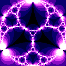
 Here are four circles inverted about each other. This is kind of similar to a Wada Basin but not exactly. Notice the small Poincar� hyperbolic tilings throughout the picture. Click here to download a Mathematica notebook for this animation. Click here to download some POV-Ray code. Here is some Mathematica code:
(* runtime: 0.3 second *) chains = {N[Append[Table[{{2E^(I theta), Sqrt[3]}}, {theta, Pi/6, 3Pi/2, 2Pi/3}], {{0, 2 - Sqrt[3]}}]]}; Reflect[{z2_, r2_}, {z1_, r1_}] := Module[{a = r1^2/((z2 -z1)Conjugate[z2 - z1] - r2^2)}, {z1 + a (z2 - z1), a r2}]; Do[chains = Append[chains, Table[Map[Reflect[#, chains[[1, j, 1]]] &, Flatten[Delete[chains[[i]], j], 1]], {j, 1, 4}]], {i, 1, 6}]; Show[Graphics[Table[{GrayLevel[i/7], Map[Disk[{Re[#[[1]]], Im[#[[1]]]}, #[[2]]] &, chains[[i]], {2}]}, {i, 1, 7}], AspectRatio -> 1, PlotRange -> {{-1, 1}, {-1, 1}}]] Another way to generate the Apollonian gasket is to use Descartes' theorem to find fourth tangent circles, given any three tangent circles. Links Apollonian - 3D shadertoy by I�igo Quilez Circle Inversion Java applet - by Pat Hooper Apollonian Gasket - by Paul Bourke Apollonian movie - by David Dumas F# code for AutoCAD - by Kean Walmsley Common Lisp code - by Luis Fallas |
3D Apollonian Fractal - ApolFrac, 8/12/09
 Given any four tangent spheres, you can find fifth tangent spheres using the Soddy-Gosset theorem, which is a generalized extension of Descartes' theorem to higher dimensions.
I haven't learned how to create this fractal on my own yet (I used ApolFrac software to create this image). Links ApolFrac - free software for 3D Apollonian spheres fractals, by Thomas Bonner F# code for AutoCAD - by Kean Walmsley, see also this version that uses a cloud-based web-service Sphere Packings in 3D - by Jos Leys |
Hénon Map Escape Time - as seen on MathWorld, Mathematica 4.2, 6/16/04
 xn+1 = 1 - a xn2 + yn, a = 0.2
yn+1 = b xn, b = 1.01 This beautiful fractal resembles a turbulent vortex. I saw this beautiful image on MathWorld but the image quality was poor due to aliasing. All I have done here is reproduce the image with antialiasing. The Hénon Map is defined by the above equations. Here is some Mathematica code: (* runtime: 12 minutes *) Henon[{x_, y_}] := {1 - 0.2 x^2 + y, 1.01 x}; DensityPlot[Length[FixedPointList[Henon[#] &, {x, y}, 1000, SameTest -> (#[[1]]^2 + #[[2]]^2 > 100 &)]], {x, 0, 4}, {y, -4, 0}, PlotPoints -> 275, AspectRatio -> 1, Mesh -> False, Frame -> False, ColorFunction -> (Hue[1 - #] &)] |
Lorenz Attractor - POV-Ray 3.6.1, 4/10/06
 The Lorenz Attractor is a famous chaotic strange attractor. The equations were originally developed to model atmospheric convection. Here is some Mathematica code: (* runtime: 1 second *) sigma = 3; rho = 26.5; beta = 1; soln = {x[t], y[t], z[t]} /. NDSolve[{x'[t] == sigma (y[t] - x[t]), y'[t] == rho x[t] - x[t]z[t] - y[t], z'[t] == x[t] y[t] - beta z[t], x[0] == 0, y[0] == 1, z[0] == 1}, {x[t], y[t], z[t]}, {t, 0, 100}, MaxSteps -> 10000][[1]]; ParametricPlot3D[soln, {t, 0, 100}, PlotPoints -> 10000, Compiled -> False] Here is some Mathematica code to numerically solve this using the 4th order Runge-Kutta method. See also my POV-Ray code: (* runtime: 0.2 second *) sigma = 3; rho = 26.5; beta = 1; dt = 0.01; p = {0, 1, 1}; v[{x_, y_, z_}] = {sigma(y - x), rho x - x z - y, x y - beta z}; Show[Graphics3D[Line[Table[k1 = dt v[p]; k2 = dt v[p + k1/2]; k3 = dt v[p +k2/2]; k4 = dt v[p + k3]; p += (k1 + 2 k2 + 2 k3 + k4)/6, {1000}]]]] Links Chaoscope - beautiful strange attractor software by Nicolas Desprez Lorenz System Fattened Trajectory - 3D manifolds by Michael Henderson Lorenz and Modular Flows - nice renderings by Jos Leys Mathematica code - by Mark McClure Java applet - by Patrick Worfolk |
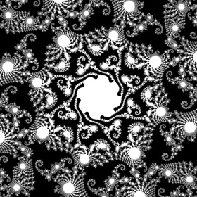
Mandelbrot Set Pickover Stalks - Mathematica 4.2, 2/24/05
 Pickover stalks are cross-shaped orbit traps invented by Clifford Pickover. See also my 3D Pickover stalks fractals. Here is some Mathematica code:
(* runtime: 33 seconds *) f[z_] := Min[Abs[{Re[z], Im[z]}]]/0.03; OrbitTrap[c_] := Module[{z = 0, i = 0}, While[i < 100 && Abs[z] < 100 && (i < 2 || f[z] > 1), z = z^2 + c; i++]; Hue[Arg[z]/(2Pi), Min[1, 2 f[z]], Max[0, Min[1, 2(1 - f[z])]]]]; Show[Graphics[RasterArray[Table[OrbitTrap[xc + I yc], {yc, -1.5, 1.5, 3/274}, {xc, -2.0, 1.0, 3/274}]], AspectRatio -> 1]] Links Biomorphs - biological-looking Pickover stalks, by Paul Bourke |
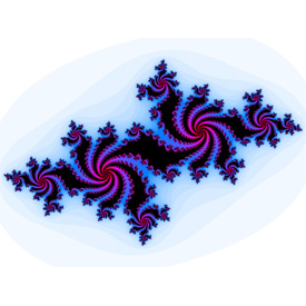
Quasifuchsian Limit Set - Mathematica 4.2, POV-Ray 3.6.1, 4/15/06
 Here is some Mathematica code for a simple Quasifuchsian limit set:
(* runtime: 15 seconds *) ta = 1.87 + 0.1I; tb = 1.87 - 0.1I; tab = (ta tb + Sqrt[ta^2tb^2 - 4(ta^2 + tb^2)])/2; z0 = (tab - 2)tb/(tb tab - 2ta + 2I tab); b = {{tb - 2I, tb}, {tb, tb + 2I}}/2; B = Inverse[b]; a = {{tab, (tab - 2)/z0}, {(tab + 2)z0, tab}}.B; A = Inverse[a]; Affine[{z1_, z2_}] := 0.01 Round[(z1/z2)/0.01]; Children[{z_, n_}] := {Affine[{a, b, A, B}[[#]].{z, 1}], #} & /@ Delete[Range[4], {3,4, 1, 2}[[n]]]; ListPlot[{Re[#[[1]]], Im[#[[1]]]} & /@ Nest[Union[Flatten[Children /@ #, 1]] &, Table[{Affine[{a, b, A, B}[[i]].{0, 1}],i}, {i, 1, 4}], 12], AspectRatio -> Automatic, PlotRange -> All] Links 3D Maskit Slices - by Kentaro Ito Fractal Field Guide - by Peter Liepa |
Crackle Fractal - Mathematica 4.2, 11/17/04
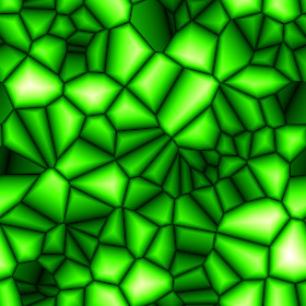
 Here is some Mathematica code for generating a periodic cellular texture based on the Voronoi diagram. This pattern resembles giraffe skin. A similar pattern can also be seen on the Netted Stinkhorn fungus. The dual of a Voronoi diagram is a Delaunay triangulation:
(* runtime: 3.8 minutes *) SeedRandom[0]; nodes = Table[Random[], {100}, {2}]; norm[x_] := x.x; Wrap[p_] := Map[If[# > 0.5, 1 - #, #] &, p]; DensityPlot[Module[{rlist = Sort[Map[norm[Wrap[Abs[# - {x, y}]]] &, nodes]]}, rlist[[2]] - rlist[[1]]], {x, 0, 1}, {y, 0, 1}, PlotPoints -> 275, Mesh -> False, Frame -> False]; Mathematica’s ComputationalGeometry package can be used to generate Voronoi diagrams: (* runtime: 1.3 seconds *) << DiscreteMath`ComputationalGeometry`; SeedRandom[0]; nodes = Table[Random[], {100}, {2}]; DiagramPlot[nodes, PlotRange -> {{0, 1}, {0, 1}}] POV-Ray has a built-in function for the crackle fractal: // runtime: 0.5 second camera{orthographic location <0,0,-4> look_at 0 angle 90} plane{z,0 pigment{crackle color_map{[0 rgb 0][0.5 rgb <0,1,0>][1 rgb 1]}} finish{ambient 1}} Links Beijing National Aquatics Center ("Water Cube") - built from ETFE for the 2008 Olympics Cellular Portrait - Java applet by Paul Chew, see also Golan Levin's Cellular Portraits Cellular Texture Tutorial - by Jim Scott Cellular Effect - by I�igo Quilez |
Mandelbrot Set Height Field - Mathematica 4.2, MathGL3d, 10/17/04
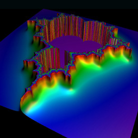 This Mandelbrot set height field was interpolated using Bill Rood’s formula for continuous escape time (cet) as described in the book “The Colours of Infinity” (see also Normalized Iteration Count Algorithm (NICA)). Here is some Mathematica code:
cet = n + log2ln(R) - log2ln|z| (* runtime: 3 seconds *) R = 6; image = ParametricPlot3D[Module[{z = 0.0, i = 0}, While[i < 100 && Abs[z] < R^2, z = z^2 + xc + I yc; i++]; cet = If[i != 100, i + (Log[Log[R]] - Log[Log[Abs[z]]])/Log[2], 0]; {xc, yc, 0.5Min[0.1cet, 1], {EdgeForm[], SurfaceColor[Hue[1 - 0.1cet]]}}], {xc, -2.0, 1.0}, {yc, -1.5, 1.5}, PlotPoints -> 64, Boxed -> False, Axes -> False, DisplayFunction -> Identity]; << MathGL3d`OpenGLViewer`; MVShow3D[image, MVNewScene -> True]; Link: height field fractals - by Jason Rampe |
Fractal Crown - as described on Paul Bourke’s web site, equations by Roger Bagula - Mathematica 4.2, 8/13/04
 Here is some Mathematica code for this fractal: (* runtime: 10 seconds *) n = 275; a = 5.0; b = Log[2]/Log[3]; image = Table[0, {n}, {n}]; Do[w = Sum[E^(I (-a)^k t)/a^(b k), {k, 1, 14}]; {i, j} = Floor[n({Re[w], Im[w]}/1.25 + 0.5)]; image[[i, j]] = Abs[w], {t, -Pi, Pi, 0.001}]; ListDensityPlot[image, Mesh -> False, Frame -> False] This is how you can make this fractal in POV-Ray: // runtime: 2 seconds camera{location <0,0,1.25> look_at 0} #macro Exp(Z) exp(Z.x)* #declare a=5; #declare b=ln(2)/ln(3); #declare t1=-pi; #while(t1 |
Bifurcation Diagram (Feigenbaum Fractal) - Mathematica 4.2, 10/17/02
 This fractal is based on the logistic equation:
xn+1 = a xn (1 - xn) Here is some Mathematica code: (* runtime: 1 minute *) Logistic[x_] := a x (1 - x); plist = {}; Do[x = 0.25; Do[x = Logistic[x], {100}]; Do[x = Logistic[x]; plist = Append[plist, {a, x}], {100}], {a, 2.8, 4, 10^-2}]; ListPlot[plist] Links Feigenbaum Function - a fractal based on the bifurcation diagram 3D Mandelbrot with bifuration - by Anders Sandberg Verhulst-Mandelbrot-Bifurcation - interesting relationship between the Mandelbrot set and bifurcation diagram |
Erosion - Kiefer in Wine Glass, 3/10/13
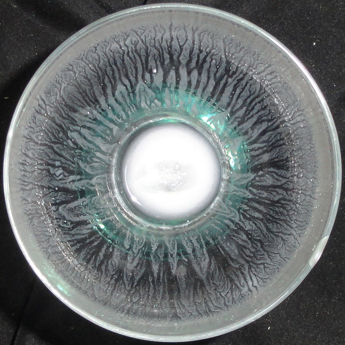 This beautiful erosion fractal emerged after I drank some kiefer from this wine glass.
 |
Circular Orbit Trap - Mathematica 4.2, 2/24/05

 This animation shows a circular orbit trap transforming into Pickover stalks. See also my 3D orbit trap fractals. Here is some Mathematica code:
(* runtime: 12 seconds *) OrbitTrap[c_] := Module[{z = 0, i = 0, x}, While[i < 10 && Abs[z] < 2 && (i < 2 || Abs[z] > 0.3), z = z^2 + c; i++]; x = Abs[z]^2/0.3^2; Hue[Arg[z]/(2Pi), Min[1, 2 x], Max[0, Min[1, 2(1 - x)]]]]; Show[Graphics[RasterArray[Table[OrbitTrap[xc + I yc], {yc, -1.5, 1.5, 3/274}, {xc, -2.0, 1.0, 3/274}]], AspectRatio -> 1]] |
Want to see more? Click here to see more fractals along with Mathematica code:
 |
More Fractals |
Fractals Links
Annual Fractal Art Contest
Felix Hausdorff - the Hausdorff dimension. He was a Jewish scientist who sadly commited suicide to avoid being taken to concentration camp.
Subdivided Columns - formed from 2700 slices of laser cut cardboard, by Michael Hansmeyer
The Art of Mathematics - fractal slideshow narrated by Lasse Rempe
Summary of Fractal Types - a long list by Noel Giffin