


Here are some more fractals, along with Mathematica code. Click here to return to the main fractals page.
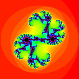
Magnet Fractals - Mathematica 4.2: 6/26/04, POV-Ray 3.6.1: 7/4/06
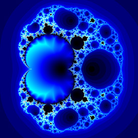
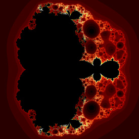 These fractals were originally designed for predicting magnetic phase-transitions. Here is some Mathematica code:
Mandelbrot[c_] := Length[FixedPointList[f[#, c] &, 0, 100, SameTest -> (Abs[#] > 2 &)]]; Magnet[] := DensityPlot[Log[Mandelbrot[xc + I yc]], {xc, -1, 3}, {yc, -2, 2}, PlotPoints -> 275, Mesh -> False, Frame -> False, ColorFunction -> (If[# != 1, Hue[#], RGBColor[0, 0, 0]] &)]; (* Magnet 1: runtime: 5 minutes *) f[z_, c_] := (z^2 + c - 1.0)^2 / (2 z + c - 2)^2; Magnet[] (* Magnet 2: runtime: 15 minutes *) f[z_, c_] := (z^3 + 3 (c - 1) z + (c - 1) (c - 2))^2 / (3 z^2 + 3 (c - 2) z + (c - 1) (c - 2) + 1.0)^2; Magnet[] POV-Ray has a built-in function for these fractals: //Magnet 1: runtime: 0.5 second camera{orthographic location <1.25,0,-2> look_at <1.25,0,0> angle 90} plane{z,0 pigment{magnet 1 mandel 50 interior 1,1 color_map{[0 rgb 0][1/6 rgb <0,0,1>][1/3 rgb 1]}} finish{ambient 1}} //Magnet 2: runtime: 0 seconds camera{orthographic location <1,0,-2> look_at <1,0,0> angle 90} plane{z,0 pigment{magnet 2 mandel 50 color_map{[0 rgb 0][1/6 rgb <1,0,0>][1/3 rgb 1][1 rgb 1][1 rgb 0]}} finish{ambient 1}} |
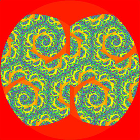
Frequency Filtered Random Noise - Mathematica 4.2, 2/12/05
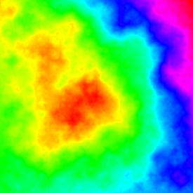
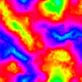 Here is another variation of frequency filtered random noise. Here is some Mathematica code:
(* runtime: 20 seconds *) n = 275; SeedRandom[1]; fourier = Fourier[Table[Random[], {n}, {n}]]; filter = Table[fourier[[i, j]]/((j/n - 0.5)^2 + (i/n - 0.5)^2), {i, 1, n}, {j, 1, n}]; ListDensityPlot[Map[Abs, InverseFourier[filter], {2}], Mesh -> False, Frame -> False, ColorFunction -> (Hue[# + 0.5] &)] |
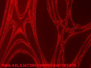
Fire Animation - adapted from Terry Robb’s Mathematica notebook, Mathematica 4.2, 12/5/04
 This texture is randomly generated to look like fire. It is not a model of real fire. Here is some Mathematica code:
(* runtime: 10 minutes *) n = 275; m = 14; SeedRandom[0]; noise = Table[Random[], {m}]; Fire[x_, y_, t_] := Module[{x2, y2, i, j, cx, cy, vx, vy, k, z = 0.0}, Do[x2 = 2^l(4.0 x - 0.01t); y2 = 2^l (2.0y - 0.1t); j = Floor[x2]; i = Floor[y2]; cx = (3 - 2(x2 - j))(x2 - j)^2; cy = (3 - 2(y2 - i))(y2 - i)^2; k = Floor[2^15 noise[[Mod[i, m] + 1]]]; vx = noise[[Mod[j + k, m] + 1]]; vy = vx + cx(noise[[Mod[j + 1 + k, m] + 1]] - vx); k = Floor[2^15 noise[[Mod[i + 1, m] + 1]]]; vx = noise[[Mod[j + k, m] + 1]]; z += Abs[vy + cy(vx + cx(noise[[Mod[j + 1 + k, m] + 1]] - vx) - vy) - 0.5]/2^l, {l, 0, 4}]; z - 0.5y]; Do[DensityPlot[Fire[x, y, t], {x, 0, 1}, {y, 0, 1}, PlotPoints -> n, Mesh -> False, Frame -> False], {t, 0, 15}]; Here is some Mathematica code to find fire color as a function of temperature. You can read more about this on Hugo Elias’ website and Henrik Jensen’ website. h = 6.62606876*^-34; c = 299792458; k = 1.380658*^-23; nm = 10^-9; FireColor[T_] := RGBColor @@ Map[Max[0, Min[1, 1 -Exp[-50*2.67253*^-13If[T < 50, 0, 2Pi h c^2/(#^5(E^(h c/(k T #)) - 1))]]]] &, {700nm, 560nm, 470nm}]; DensityPlot[x, {x, 0, 1}, {y, 0, 1/6}, AspectRatio -> Automatic, PlotPoints -> {275, 2}, Mesh -> False,Frame -> False, ColorFunction -> (FireColor[6023#] &)] |
Lambda Fractal - as seen on http://www.math.utsa.edu/mirrors/maple/mfrlbd.htm, Mathematica 4.2, 6/26/04
 This fractal is based on a complex version of the logistic equation. Here is some Mathematica code:
zn+1 = a zn(1 - zn), a = 0.85 + 0.6 i (* runtime: 38 seconds *) Julia = Compile[{{z, _Complex}}, Length[FixedPointList[f, z, 50, SameTest -> (Abs[#] > 2 &)]]]; f[z_] := c z(1 - z); c = 0.85 + 0.6 I; DensityPlot[Julia[x + I y], {x, -1, 2}, {y, -1.5, 1.5}, PlotPoints -> 275, Mesh -> False, Frame -> False, ColorFunction -> (If[# != 1, Hue[#], Hue[0, 0, 0]] &)] |
Barnsley’s Tree Julia Set Fractal - as seen on MathWorld, Mathematica 4.2, 6/11/04
 zn+1 = c(zn - sign(Re(zn))), c = 0.6+1.1i
Here is some Mathematica code for this fractal: (* runtime: 38 seconds *) Julia = Compile[{{z, _Complex}}, Length[FixedPointList[f, z, 100, SameTest -> (Abs[#] > 2 &)]]]; f[z_] := c(z - Sign[Re[z]]); c = 0.6 + 1.1 I; DensityPlot[Julia[x + I y], {x, -2, 2}, {y, -2, 2}, PlotPoints -> 275, Mesh -> False, Frame -> False, ColorFunction -> Hue] |
Spiral-Shaped Julia Set Fractal - Mathematica 4.2, 3/14/04
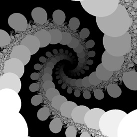 zn+1 = tan(zn2 + c), c = 2.0625+0.1425i
Here is some Mathematica code for this fractal: (* runtime: 5 minutes *) Julia = Compile[{{z, _Complex}}, Length[FixedPointList[f, z, 250, SameTest -> (Abs[#] > 2 &)]]]; f[z_] := Tan[z^2 + c]; c = 2.0625 + 0.1425 I; DensityPlot[Log[Julia[x + I y]], {x, 0.64836364, 0.92763636}, {y, 1.20509091, 1.48872727}, PlotPoints -> 275, Mesh -> False, Frame -> False, ColorFunction -> (CMYKColor[#, #, #, 0] &)] |
Arrowhead-Shaped Mandelbrot Set Fractal - Mathematica 4.2, 2/3/02
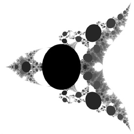 zn+1 = tan(zn2+c)
Here is some Mathematica code for this fractal: (* runtime: 5 minutes *) Mandelbrot[c_] := Length[FixedPointList[f[#, c] &, 0, 100, SameTest -> (Abs[#] > 2 &)]]; f[z_, c_] := Tan[z^2 + c]; DensityPlot[Log[Mandelbrot[xc + I yc]], {xc, 0.2, 3.3}, {yc, -1.55, 1.55}, PlotPoints -> 275, Mesh -> False, Frame -> False] |
Curlicue Fractal for the Feigenbaum Constant, Mathematica 4.2, 6/11/04
 Here is some Mathematica code for a Curlicue Fractal:
(* runtime: 0.15 second *) s = 4.669201609102990; ListPlot[{Re[#], Im[#]} & /@ FoldList[Plus, 0, Exp[I Pi s Range[10000]^2]], PlotJoined -> True, AspectRatio -> Automatic, Axes -> None] Link: Fergus Ray-Murray’s Curlicue Fractals |
Plasma Fractal - adapted from Justin Seyster’s Plasma Java applet, 8/16/04
 This Mathematica code generates non-periodic random textures using a bisection method. This is another popular technique for generating terrain.
(* runtime: 19 seconds *) n = 256; image = Table[0, {n}, {n}]; Plasma[w_, {x_, y_}, {{a_, c_}, {g_, i_}}] := If[w < 2, image[[y + 1, x + 1]] = (a + c + g + i)/4, Module[{b = (a + c)/2, d = (a + g)/2, e = Min[Max[(a + c + g + i)/4 + 1.5 (Random[] - 0.5) w/n, 0], 1], f = (c + i)/2, h = (g + i)/2}, Plasma[w/2, {x, y}, {{d, e}, {g, h}}]; Plasma[w/2, {x + w/2, y}, {{e, f}, {h, i}}]; Plasma[w/2, {x, y + w/2}, {{a, b}, {d, e}}]; Plasma[w/2, {x + w/2, y + w/2}, {{b, c}, {e, f}}]]]; Plasma[n, {0, 0}, Table[Random[], {2}, {2}]]; ListDensityPlot[image, Mesh -> False, Frame -> False, ColorFunction -> Hue] |
Koch’s Snowflake - AutoCAD, AutoLisp, 10/25/00
 This is another type of L-System.
Links The self-similar rippling of leaf edges and torn plastic sheets - hyperbolic surfaces resembling Koch’s snowflake L-Systems - Mathematica code by unknown author, hosted by Jan Poland |
Web - Java applet, 5/22/01
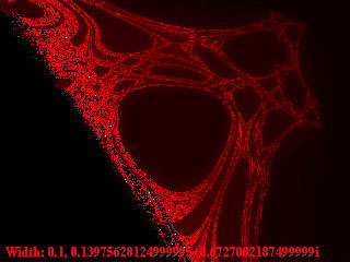
 This was the first “complex” fractal I ever made. I accidentally made this fractal while trying to generate the Mandelbrot set. Unfortunately, I don’t remember how to make it. Please let me know if you figure it out! I think the original code went something like this:
(* runtime: 38 seconds *) Web[xc_, yc_] := Module[{x = 0, y = 0, i = 0}, While[i < 100 && (x^2 + y^2) < 4, x = x^2 - y^2 + xc; y = 2x y + yc; i++]; i]; DensityPlot[Log[Web[xc, yc]], {xc, -2, 1}, {yc, -1.5, 1.5}, PlotPoints -> 275, Mesh -> False, Frame -> False, ColorFunction -> (If[# == 1, Hue[0, 0, 0], Hue[0,Min[1, 2(1 - #)], Min[1, 2#]]] &)] |