


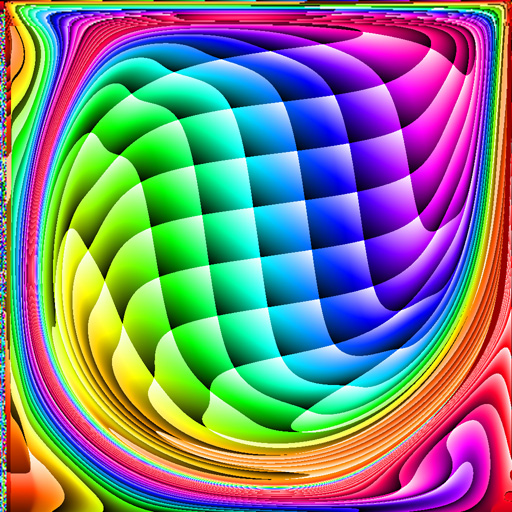
Water Ripple Simulation - calculated in Mathematica 4.2, 12/2/04; rendered in POV-Ray 3.6.1, 7/29/05
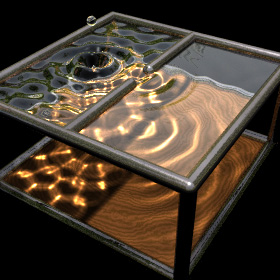

 Here is a simple water ripple simulation showing single slit wave diffraction. The following Mathematica code solves the wave equation with damping using the finite difference method. You can read more about this algorithm on Hugo Elias’ website. (Note: technically this simulation should use Neumann boundary conditions but I decided it was simpler to demonstrate using Dirichlet boundary conditions). See also the Shallow Water Equation. (* runtime: 18 seconds, c is the wave speed and b is a damping factor *) n = 64; c = 1; b = 5; dx = 1.0/(n - 1); Courant = Sqrt[2.0]/2;dt = Courant dx/c; z1 = z2 = Table[0.0, {n}, {n}]; Do[{z1, z2} = {z2, z1}; z1[[n/2, n/4]] = Sin[16Pi t]; Do[If[0.45 < i/n < 0.55 || ! (0.48 < j/n < 0.52), z2[[i, j]] = z1[[i, j]] + (z1[[i, j]] - z2[[i, j]] + Courant^2 (z1[[i - 1, j]] + z1[[i + 1, j]] + z1[[i, j - 1]] + z1[[i, j + 1]] - 4 z1[[i, j]]))/(1 + b dt)], {i, 2, n - 1}, {j, 2, n - 1}]; ListPlot3D[z1, Mesh -> False, PlotRange -> {-1, 1}], {t, 0, 1, dt}]; Links LSSM - POV-Ray animations using this same technique, by Tim Nikias Wenclawiak POV-Ray Ripples - another one by Rune Johansen Water Ripples - Delphi program by Jan Horn Waves - C++ program by Maciej Matyka |
Unstable Vortex Filaments - C#, POV-Ray 3.6.1, 9/6/12
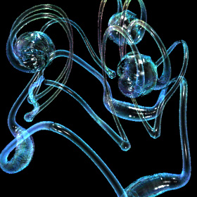
 Here is a simulation of two unstable leap-frogging vortex filaments in 3D, assuming inviscid incompressible potential flow. The vortex filaments were simulated using the Biot-Savart law for vortex segments. Here is some Mathematica code:
(* runtime: 38 seconds *) abs[x_] := Sqrt[x.x]; Normalize[x_] := x/abs[x]; Mean[x_] := Plus @@ x/Length[x]; v[p_] := Module[{v = 0.0}, Scan[({p1,p2} = #; r12 = p2 - p1; zhat = Normalize[r12]; r0 = p1 - p + (p - p1).zhat zhat; r = abs[r0]; If[r > 0.001, gamma = 1.0/abs[r12]; rcore = 0.15Sqrt[gamma]; rhat = Normalize[r0]; cos1 = rhat.Normalize[p1 - p]; cos2 = rhat.Normalize[p2 - p]; thetahat = Cross[zhat, rhat]; v += (gamma/r)(1 - Exp[-(r/rcore)^2])(cos1 + cos2)thetahat]) &, Partition[filament, 2, 1, 1]]; v]; dt = 0.001; filament = Table[{Cos[theta], Sin[theta], 0.0}, {theta, 0.0, 2Pi - 0.001, Pi/18}]; Do[filament = Map[(# + v[#] dt) &, filament]; If[t > 190, p0 = Mean[filament]; Show[Graphics3D[Line[Map[# - p0 &, filament]], PlotRange -> 2{{-1, 1}, {-1, 1}, {-1, 1}}]]], {t, 1, 230}] Links Vortex Movies - by Tee Tai Lim, I especially like the movies of leap-frogging and vortex ring collisions Turbulence Infinite - a single incredibly knotted vortex filament, by Mark Stock Fuzzy Smoke - vortex filament simulation, by Daniel Piker |
Leap-Frogging Bubble Rings - Mathematica 4.2, POV-Ray 3.6.1, 12/31/05
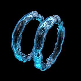
 Here is a pair of leap-frogging bubble rings.
Links Extraordinary Toroidal Vortices - popular YouTube video that uses my animation, Chris M. Bubble Ring Videos - blown by human, whale, dolphins. This is fun... try it some time! Leap-Frogging Bubble Rings - blown by scuba diver Bubble Rings - by David Whiteis Vortex rings blown out by Mt. Etna - same as a smoker puffing out an “O” ring Smoke Ring - giant vortex ring at the Miramar Air Show Zero Blaster - fun toys that create fog vortex rings Ideal Flow Machine - Java applet by William Devenport Inviscid Flows - paper on incompressible, irrotational flows by Paul Hammerton |
Leap-Frogging Vortices - Mathematica 4.2 version: 12/31/05; C++ version: 10/22/07


 Here is a simple technique for modeling 2D vortices assuming inviscid incompressible potential flow (irrotational). This technique was inspired from Kerry Mitchell’s paper based on Ultra Fractal. Here is some Mathematica code to plot the entrained fluid: (* runtime: 25 seconds, increase n for better resolution *) tmax = 0.85; rcore = 0.1; Klist = {1, -1, 1, -1}; zlist0 = {-1 - 0.5I, -1 + 0.5I, -0.5 - 0.5I, -0.5 + 0.5I}; m = Length[zlist0]; v[K_, z_, z0_] := Module[{r2 = Abs[z - z0]^2}, I K(z0 - z)/r2(1 - Exp[-r2/rcore^2])]; zlist = NDSolve[Flatten[Table[{Subscript[z,i]'[t] == Sum[If[i == j, 0, v[Klist[[j]], Subscript[z, i][t], Subscript[z, j][t]]], {j, 1, m}], Subscript[z, i][0] ==zlist0[[i]]}, {i, 1, m}]], Table[Subscript[z, i][t], {i, 1, m}], {t, 0, tmax}][[1, All, 2]]; n = 23; image = Table[NDSolve[{z'[t] == Sum[v[Klist[[i]], z[t], zlist[[i]]], {i, 1, m}], z[tmax] == x + I y}, z[t], {t, 0, tmax}, MaxSteps -> 5000][[1, 1, 2]] /. t -> 0, {y, -1.125, 1.125, 2.25/n}, {x, -0.35, 1.9, 2.25/n}]; ListDensityPlot[Map[Sign[Im[#]]Arg[#] &, image, {2}], Mesh -> False, Frame -> False, AspectRatio -> Automatic] Here is some Mathematica code to numerically solve this using the 4th order Runge-Kutta method: (* runtime: 21 seconds, increase n for better resolution *) n = 23; tmax = 0.85; dt = tmax/100; rcore = 0.1; Klist = {1, -1, 1, -1}; zlist = {-1 - 0.5I, -1 + 0.5I, -0.5 - 0.5I, -0.5 + 0.5I}; m = Length[zlist]; v[K_, z_, z0_] := Module[{r2 = Abs[z - z0]^2}, I K(z0 - z)/r2(1 - Exp[-r2/rcore^2])]; Runge[z_] := Module[{}, k1 = dt vtot[z]; k2 = dt vtot[z + k1/2]; k3 = dt vtot[z + k2/2]; k4 = dt vtot[z + k3]; (k1 + 2 k2 + 2 k3 + k4)/6]; vtot[zlist_] := Table[Sum[If[i == j, 0, v[Klist[[j]], zlist[[i]], zlist[[j]]]], {j, 1, m}], {i, 1, m}]; zlists = Transpose[Table[zlist += Runge[zlist], {t, 0, tmax, dt}]]; vtot[z_] := Plus @@ v[Klist, z, zlists[[All, t]]]; image = Table[z = x + I y; Do[z -= Runge[z], {t, 100, 1, -1}]; z, {y, -1.125, 1.125, 2.25/n}, {x, -0.35, 1.9, 2.25/n}]; ListDensityPlot[Map[Sign[Im[#]]Arg[#] &, image, {2}], Mesh -> False, Frame -> False, AspectRatio -> Automatic] Links YouTube animation - a very similar looking animation My Educational Project - some basic potential flows using Matlab and Mathematica Nuclear Bombs - mushroom clouds are giant vortex rings Birth of the Jellyfish - nice animation by Kerry Mitchell |
Driven Cavity - calculated in Fortran 90, plotted in Mathematica 4.2, 11/2/05


 Here is the flow inside a square box where the flow across the top of the box is moving to the right at Reynolds number 1000. This program uses the finite volume method to solve the Navier-Stokes equations assuming steady, incompressible, viscous, laminar flow. This was calculated on a 300�300 non-uniform grid and took 3 hours to run on my laptop. The animation shows the motion along the streamlines/pathlines. The following Mathematica code is not completely accurate at the boundaries, but it gives the basic idea:
(* runtime: 20 minutes *) n = 50; dx = 1.0/(n - 1); RE = 1000; relax = 0.4; residu = residv = residp = 1; u = Table[If[j == 1 || i == 2 || i == n, 0, 1], {i, 1, n}, {j, 1, n}]; v = p = pstar = ap = an = as = aw = ae = sc = sp = du = dv = Table[0, {n}, {n}]; lisolv[i0_, j0_, phi0_] := Module[{phi = phi0, p = q =Table[0, {n}]}, Do[q[[j0 - 1]] = phi[[i, j0 - 1]]; Do[p[[j]] = an[[i, j]]/(ap[[i, j]] -as[[i, j]]p[[j - 1]]); q[[j]] = (as[[i, j]]q[[j - 1]] + ae[[i, j]] phi[[i + 1, j]] + aw[[i, j]]phi[[i - 1, j]] + sc[[i, j]])/(ap[[i, j]] - as[[i, j]]p[[j - 1]]), {j, j0, n - 1}]; Do[phi[[i,j]] = p[[j]]phi[[i, j + 1]] + q[[j]], {j, n - 1, j0, -1}], {i, i0, n - 1}]; phi]; calc[i0_, j0_] := Module[{}, {cn, cs, ce, cw} = 0.5 {v[[i,j + 1]] + v[[i0, j0 + 1]], v[[i, j]] + v[[i0, j0]], u[[i + 1, j]] + u[[i0 + 1, j0]], u[[i, j]] + u[[i0, j0]]}dx; cp = Max[0, cn - cs + ce - cw]; {an[[i, j]], as[[i, j]], ae[[i, j]], aw[[i, j]]} = Map[Max[0, 1 - 0.5 Abs[#]] &, RE{cn, cs, ce, cw}]/RE + Map[Max[0, #] &, {-cn, cs, -ce, cw}]; sp[[i, j]] = -cp; ap[[i, j]] = an[[i, j]] + as[[i, j]] + ae[[i, j]] + aw[[i, j]] - sp[[i, j]]]; While[Max[residu, residv, residp] > 0.001, residu = residv = residp = 0; Do[calc[i - 1, j]; sc[[i, j]] = cp u[[i, j]] + dx(p[[i - 1, j]] - p[[i, j]]); du[[i, j]] = relax dx/ap[[i, j]]; residu += Abs[an[[i, j]]u[[i, j + 1]] + as[[i, j]]u[[i, j - 1]] + ae[[i, j]]u[[i + 1, j]] + aw[[i, j]]u[[i - 1, j]] - ap[[i, j]]u[[i, j]] + sc[[i, j]]], {i, 3, n - 1}, {j, 2, n - 1}]; ap /= relax; sc += (1 - relax) ap u; u = lisolv[3, 2, u]; Do[calc[i, j - 1]; sc[[i, j]] = cp v[[i, j]] + dx(p[[i, j - 1]] - p[[i, j]]); dv[[i, j]] = relax dx/ap[[i, j]];residv += Abs[an[[i, j]]v[[i, j + 1]] + as[[i, j]]v[[i, j - 1]] + ae[[i, j]]v[[i + 1, j]] + aw[[i, j]]v[[i - 1, j]] - ap[[i, j]]v[[i, j]] + sc[[i, j]]], {i, 2, n - 1}, {j, 3, n - 1}]; ap /= relax; sc += (1 - relax)ap v; v = lisolv[2, 3, v];Do[an[[i, j]] = dx dv[[i, j + 1]]; as[[i, j]] = dx dv[[i, j]]; ae[[i, j]] = dx du[[i + 1, j]]; aw[[i, j]] = dx du[[i, j]]; sp[[i, j]] = 0; sc[[i, j]] = -((v[[i, j + 1]] - v[[i, j]])dx + (u[[i + 1, j]] - u[[i, j]]) dx); residp += Abs[sc[[i, j]]]; ap[[i, j]] = an[[i, j]] + as[[i, j]] + ae[[i, j]] + aw[[i, j]] - sp[[i, j]]; pstar[[i, j]] = 0, {i, 2, n - 1}, {j, 2, n - 1}]; Do[pstar = lisolv[2, 2, pstar], {2}]; Do[If[i != 2, u[[i, j]] += du[[i, j]](pstar[[i - 1, j]] - pstar[[i, j]])]; If[j != 2, v[[i, j]] += dv[[i, j]](pstar[[i, j - 1]] - pstar[[i, j]])]; p[[i, j]] += 0.3(pstar[[i, j]] - pstar[[n - 1, n - 1]]), {i, 2, n - 1}, {j, 2, n - 1}]]; |

 Here is some Mathematica code to plot streamlines. The blue lines are rotating clockwise and the red lines are rotating counter-clockwise. The plot on the left agrees fairly well with Ercan Erturk’s results. psi = Table[0, {n - 1}, {n - 1}]; Do[psi[[i, j]] = psi[[i, j - 1]] + dx(u[[i + 1, j - 1]] + u[[i + 1, j]])/2, {j, 2, n - 1}, {i, 1, n - 1}]; psi = ListInterpolation[psi, {{0, 1}, {0, 1}}]; ContourPlot[psi[x, y], {x, 0, 1}, {y, 0, 1}, PlotPoints -> 50, PlotRange -> All, ContourShading -> False,Contours -> {-0.08, -0.077, -0.07, -0.06, -0.045, -0.025, -0.01, -0.0025, 0, -8*^-6, 2*^-6, 3*^-5, 8*^-5, 1*^-4, 3*^-4, 6*^-4, 9*^-4}, ContourStyle -> Table[{Hue[2(1 - x)/3]}, {x, 0, 1, 1/16}]] |

 Here is some Mathematica code to plot vorticity contours. The plot on the left agrees fairly well with Ghia’s results. omega = ListInterpolation[Table[(v[[i, j]] - v[[i - 1, j]])/dx - (u[[i, j]] - u[[i, j - 1]])/dx, {i, 2, n - 1}, {j, 2, n - 1}], {{0, 1}, {0, 1}}]; ContourPlot[omega[x, y], {x, 0, 1}, {y, 0, 1},PlotPoints -> 50, PlotRange -> All, ContourShading -> False, Contours -> Range[-14, 7],ContourStyle -> Table[{Hue[2(1 - x)/3]}, {x, 0, 1, 1/21}]] Computational Fluid Dynamics (CFD) Links CFD Gallery - by Arthur Veldman, I especially like the simulations of turbulence Turbulent Boundary Layer - large simulation by Said Elghobashi Colorful Fluid Mixing Gallery - by Andr� Bakker CFD code - simple Fortran codes by Abdusamad Salih FlowLab - educational resource by Fluent |
Driven Cavity - Mathematica 4.2, 11/16/06
|
Here is the same driven cavity using the finite difference method. This code uses the Alternating Direction Implicit (ADI) method to solve the vorticity transport equation assuming unsteady, incompressible, viscous flow. This method seems to be much faster and easier to implement in this case than the finite volume method. (* runtime: 1 minute *) << LinearAlgebra`Tridiagonal`; n = 20; RE = 1000; dx = 1.0/(n - 1); dt = 0.25; cxy = dt/(4dx); sxy = dt/(2RE dx^2); lambda = 1.5; free = Range[2, n - 1]; omega = v = psi = Table[0, {n}, {n}]; u = Table[If[j == n, 1, 0], {n}, {j, 1, n}]; Do[omega[[All, 1]] = 2psi[[All, 2]]/dx^2; omega[[All, n]] = 2 (psi[[All, n - 1]] + dx)/dx^2; omega[[1, All]] = 2 psi[[2, All]]/dx^2; omega[[n, All]] = 2 psi[[n - 1, All]]/dx^2; omega[[free, free]] = Transpose[Partition[TridiagonalSolve[Drop[Flatten[Table[If[i == n - 1, 0, -(cxy u[[i, j]] + sxy)], {j, 2, n - 1}, {i, 2, n - 1}]], -1], Flatten[Table[1 + 2sxy, {j, 2, n - 1}, {i, 2, n - 1}]], Drop[Flatten[Table[If[i == n - 1,0, cxy u[[i + 1, j]] - sxy], {j, 2,n - 1}, {i, 2, n - 1}]], -1], Flatten[Table[(cxy v[[i, j - 1]] + sxy)omega[[i, j - 1]] + (1 - 2sxy)omega[[i, j]] + (-cxy v[[i, j + 1]] + sxy)omega[[i, j + 1]] + If[i == 2, (cxy u[[i - 1, j]] + sxy)omega[[i - 1, j]],0] - If[i == n - 1, (cxy u[[i + 1, j]] - sxy) omega[[i + 1, j]], 0], {j, 2, n - 1}, {i, 2, n - 1}]]], n - 2]]; omega[[free, free]] = Partition[TridiagonalSolve[Drop[Flatten[Table[If[j == n - 1, 0, -(cxy v[[i, j]] + sxy)], {i, 2, n - 1}, {j, 2, n - 1}]], -1], Flatten[Table[1 + 2sxy, {i, 2, n - 1}, {j, 2, n - 1}]], Drop[Flatten[Table[If[j == n - 1, 0, cxy v[[i, j + 1]] - sxy], {i, 2, n - 1}, {j, 2, n - 1}]], -1], Flatten[Table[(cxy u[[i - 1, j]] + sxy)omega[[i - 1, j]] + (1 - 2sxy)omega[[i, j]] + (-cxy u[[i + 1, j]] +sxy)omega[[i + 1, j]] + If[j == 2, (cxy v[[i, j - 1]] + sxy)omega[[i, j - 1]], 0] - If[j == n - 1, (cxy v[[i, j + 1]] - sxy) omega[[i, j + 1]], 0], {i, 2, n - 1}, {j, 2, n - 1}]]], n - 2]; resid = 1; While[resid > 0.001, resid = 0; Do[resid += Abs[psi[[i, j]] - (psi[[i,j]] = lambda(psi[[i, j - 1]] + psi[[i - 1, j]] + psi[[i + 1, j]] + psi[[i, j + 1]] - dx^2omega[[i, j]])/4 + (1 - lambda)psi[[i, j]])], {i, 2, n - 1}, {j, 2, n - 1}]]; Do[u[[i, j]] = (psi[[i, j + 1]] - psi[[i, j - 1]])/(2dx); v[[i, j]] = -(psi[[i + 1, j]] - psi[[i - 1, j]])/(2dx), {i, 2, n - 1}, {j, 2, n - 1}]; ListContourPlot[Transpose[psi], PlotRange -> All, ContourShading -> False], {100}]; Link: Driven Cavity - simple Fortran program by Zheming Zheng that uses this method |
2D Smoothed Particle Hydrodynamics (SPH) - calculated in C++, rendered in POV-Ray 3.6.1, 12/10/08
 The following Mathematica code for 2D SPH uses the same kernal functions as the 3D code:
(* runtime: 6.4 minutes *) Norm[x_] := x.x; PlotColor[x_] := Hue[2(1 - Min[1, Max[0, x]])/3]; dt = 0.004; g = {0, -9.8}; mu = 0.2; rho0 = 600; m = 0.00020543; r0 = 0.004; rsmooth = 0.01; rsmooth2 = rsmooth^2; vmax = 200; vmax2 = vmax^2; WPoly6Kernal = 315/(64Pi rsmooth^9); SpikyKernal = -45/(Pi rsmooth^6); LaplacianKernal = 45/(Pi rsmooth^6); IntStiff = 0.5; ExtStiff = 20000; damp = 256; p = 1; v = 2; v2 = 3; F = 4; P = 5; nu = 6; xmax = 0.1; dx = 0.87(m/rho0)^(1/3); particles = Flatten[Table[{{x, y}, {0, 0}, {0, 0}, {0, 0}, 0, 0}, {y, -xmax, 0,dx}, {x, 0, xmax, dx}], 1]; n = Length[particles]; Do[Do[rho = WPoly6Kernal m Sum[If[i != j, Max[0, (rsmooth2 - Norm[particles[[i, p]] - particles[[j, p]]])^3], 0], {j, 1, n}]; particles[[i, P]] = (rho - rho0)IntStiff; particles[[i, nu]] = If[rho > 0, 1/rho, 0], {i, 1, n}];Do[A = particles[[i]]; particles[[i, F]] = Sum[If[i != j, B = particles[[j]]; dx = A[[p]] - B[[p]]; r2 = Norm[dx];If[r2 < rsmooth2, r = Sqrt[r2]; c = rsmooth - r; c A[[nu]] B[[nu]](-0.5 c SpikyKernal(A[[P]] + B[[P]])dx/r + LaplacianKernal mu(B[[v2]] - A[[v2]])), 0], 0], {j, 1, n}], {i, 1, n}];Do[A = particles[[i]]; a = A[[F]]m; If[Norm[a] > vmax2, a = vmax a/Sqrt[Norm[a]]]; Do[d = xmax - sign A[[p, dim]]; If[d < 2r0 - 0.00001, normal = {0, 0}; normal[[dim]] = -sign;a += (ExtStiff(2r0 - d) - damp normal.A[[v2]]) normal], {sign, -1, 1, 2}, {dim, 1, 2}];a += g; particles[[i, v2]] = A[[v]] + a dt/2; particles[[i, v]] = A[[v]] + a dt; particles[[i, p]] += particles[[i, v]] dt, {i, 1, n}]; Show[Graphics[Table[{PlotColor[particles[[i, P]]/1500], Point[particles[[i, p]]]}, {i, 1,n}], AspectRatio -> Automatic, PlotRange -> xmax{{-1, 1}, {-1, 1}}]], {100}] Links Fluid v1.0 - C++ program for fluid surfaces by Maciej Matyka, uses Marker And Cell (MAC) method Splash - analytical Mathematica plot by Dr. Jim Swift Particle Fluid - Java applet using a simple technique, by Chris Laurel Lobe Compressor - SPH simulation by Simerics |
3D Smoothed Particle Hydrodynamics (SPH) - calculated in C++, rendered in POV-Ray 3.6.1, 12/10/08
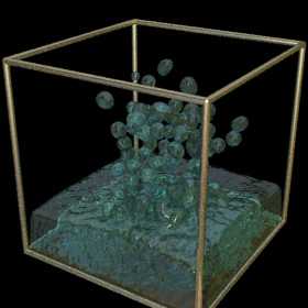 When a droplet falls into shallow water, it creates a crown or "coronet". This droplet simulation was calculated using Smoothed Particle Hydrodynamics (SPH). SPH is one of the most impressive-looking fluid simulation techniques.
Droplet Links Liquid Sculpture - beautiful high speed photographs, by Martin Waugh, see also this video Water Figures - beautiful high-speed camera splashes by Fotoopa Other Links Fluids v.3 - fast SPH C++ program by Rama Hoetzlein Physics Demos - fluid Java applets by Grant Kot Fluid Animations - amazing animations by Ron Fedkiw, with Eran Guendelman, Andrew Selle, Frank Losasso, et al. POVFlow - by Fidos GPU Fluid Solver - by Keenan Crane, uses Graphics Processing Unit (GPU) for fast calculations Free Surface Fluid Simulations - impressive simulations using the Lattice-Boltzmann method with level sets, by Nils Thuerey, author of Blender’s fluid package ball in water - nice 3D POV-Ray animation by Fidos Harmonic Fluids - simulation of fluid sounds Smoke Animations - by Jos Stam, Henrik Jensen, Ron Fedkiw, et al. Fire Animations - by Duc Nguyen, Henrik Jensen, Ron Fedkiw Bouncing liquid jets - University of Texas Mark Stock - impressive fluid simulation artwork Rune’s Particle System - nice POV-Ray program by Rune Johansen |
Von Kármán Vortex Street - C++, 1/11/05
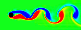
 When fluid passes an object, it can leave a trail of vortices called a Von Kármán Vortex Street. This animation shows the vorticity where blue is clockwise and red is counter-clockwise. This simulation assumes unsteady, incompressible, viscid, laminar flow. For solenoidal flows, mass conservation can be achieved by taking the Fast Fourier Transform (FFT) of the velocity and then removing the radial component of the wave number vectors. The code was adapted from Jos Stam’s C Source Code and paper which is patented by Alias. Thanks to xzczd for debugging this code. Click here to see an optimized implementation: (* runtime: 4 minutes *) n = 64; dt = 0.3; mu = 0.001; v = Table[{0, 0}, {n}, {n}]; ListAnimate@Table[Do[If[i < 5, v[[i, j]] = {0.1, 0}]; If[(i - n/4)^2 + (j - n/2)^2 < 4^2, v[[i, j]] = {0, 0}], {i, 1, n}, {j, 1, n}]; ui = ListInterpolation[v[[All, All, 1]]]; vi = ListInterpolation[v[[All, All, 2]]]; v = Table[{i2, j2} = {i, j} - n dt v[[i, j]]; {ui[i2, j2], vi[i2, j2]}, {i, 1, n}, {j, 1, n}]; v = Transpose[Map[Fourier[v[[All, All, #]]] &, {1, 2}], {3, 1, 2}]; v = Table[x = Mod[i + n/2 - 1, n] - n/2; y = Mod[j + n/2 - 1, n] - n/2; k = x^2 + y^2; Exp[-k dt mu] If[k > 0, (v[[i, j]] . {-y, x}/k) {-y, x}, v[[i, j]]], {i, 1, n}, {j, 1, n}]; v = Transpose[Map[Re[InverseFourier[v[[All, All, #]]]] &, {1, 2}], {3, 1, 2}]; ListDensityPlot[Table[((v[[i + 1, j, 2]] - v[[i - 1, j, 2]]) - (v[[i, j + 1, 1]] - v[[i, j - 1, 1]]))/2, {j, 2, n - 1}, {i, 2, n - 1}], Mesh -> False, Frame -> False, ColorFunction -> (Hue[2 #/3] &), PlotRange -> All], {t, 1, 350}] Links smoke program - uses this method, by Gustav Taxén fire program - uses this method, Hugo Elias Fluid Simulations - nice vortex street simulations by Maciej Matyka Vortex street in the clouds - photo of a vortex street created by an island Airplane Vortices - nice photo of trailing airplane vortices Harmonic Balance CFD |
Flapping Wing - Fortran 90, rendered in POV-Ray 3.6.1, 4/28/06
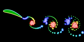
 This flapping wing was calculated using the unsteady vortex panel method adapted from Alan Lai’s Fortran code. It assumes inviscid incompressible potential flow (irrotational). I also have a Mathematica version of this code, but it is a little lengthy to show here. See also my biomimetics links.
Links Unsteady Panel Code Simulations - by Kevin Jones Insect Flight - Jane Wang made one of the first simulations to predict that an insect can produce sufficient lift to remain aloft. Here is another article about it. See also these Vortex Method Simulations by Jeff Eldredge. Robotic Fly - Uses piezoelectric actuators, by Ron Fearing. See also his Microfly with piezoelectric actuators. Harvard Microrobotics Lab - see this video Flapping MAV - interesting design by Kevin Jones |
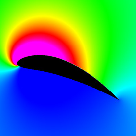
Joukowski Airfoil - C++, 11/8/07
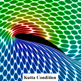
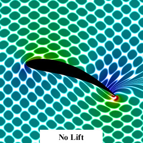

 These animations were created using a conformal mapping technique called the Joukowski Transformation. A Joukowski airfoil can be thought of as a modified Rankine oval. It assumes inviscid incompressible potential flow (irrotational). Potential flow can account for lift on the airfoil but it cannot account for drag because it does not account for the viscous boundary layer (D'Alembert's paradox). In these animations, red represents regions of low pressure. The left animation shows what the surrounding fluid looks like when the Kutta condition is applied. Notice that the fluid separates smoothly at the trailing edge of the airfoil and a low pressure region is produced on the upper surface of the wing, resulting in lift. The lift is proportional to the circulation around the airfoil. The right animation shows what the surrounding fluid looks like when there is no circulation around the airfoil (no lift). Notice the sharp singularity at the trailing edge of the airfoil. This singularity would not happen on a real airfoil. Instead the flow would separate and the airfoil would stall.
|
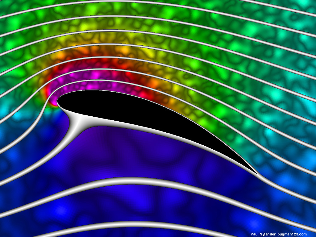
 Here is an animation that shows how the streamlines change when you increase the circulation around the airfoil. (Please note: The background fluid motion in this animation is just for effect and is not accurate!) Here is some Mathematica code to plot the streamlines and pressure using Bernoulli’s equation:
(* runtime: 13 seconds *) Clear[z]; U = rho = 1; chord = 4; thk = 0.5; alpha = Pi/9; y0 = 0.2; x0 = -thk/5.2; L = chord/4; a = Sqrt[y0^2 + L^2]; gamma = 4Pi a U Sin[alpha + ArcCos[L/a]]; w[z_, sign_] := Module[{zeta = (z + sign Sqrt[z^2 - 4 L^2])/2}, zeta = (zeta - x0 - I y0)Exp[-I alpha]/Sqrt[(1 - x0)^2 + y0^2]; U(zeta + a^2/zeta) + I gamma Log[zeta]/(2Pi)]; sign[z_] := Sign[Re[z]]If[Abs[Re[z]] < chord/2 && 0 < Im[z] < 2y0(1 - (2Re[z]/chord)^2), -1, 1];w[z_] := w[z, sign[z]]; V[z_] = D[w[z, sign], z] /. sign -> sign[z]; ContourPlot[Im[w[(x + I y)Exp[I alpha]]], {x, -3, 3}, {y, -3, 3}, Contours -> Table[x^3 + 0.0208, {x, -2, 2, 0.1}], PlotPoints -> 100, ContourShading -> False, AspectRatio -> Automatic] DensityPlot[-0.5rho Abs[V[(x + I y)Exp[I alpha]]]^2, {x, -3, 3}, {y, -3, 3}, PlotPoints -> 275, Mesh -> False, Frame -> False, ColorFunction -> (If[# == 1, Hue[0, 0, 0], Hue[(5# - 1)/6]] &), AspectRatio -> Automatic] Links Joukowski Animation - nice animation showing how the fluid moves Joukowski Airfoil - nice Java applet by NASA Nikolai Joukowski - used this technique to find the lift on an airfoil in 1906, long before modern computers |
NACA Airfoil - Mathematica 4.2, 12/16/05
 Here is a 9415 NACA airfoil. It looks similar to the Joukowski airfoil, but the shape is slightly better. Here is some Mathematica code:
(* runtime: 0.01 second *) Clear[x]; n = 40; c = 0.09; p = 0.4; t = 0.15; camber := c If[x < p, (2p x - x^2)/p^2, ((1 - 2p) + 2p x - x^2)/(1 - p)^2]; theta = ArcTan[D[camber, x]]; p = Table[x = 0.5(1 - Cos[Pi s]); x1 = 1.00893x; thk = 5t(0.2969Sqrt[x1] - 0.126x1 - 0.3516x1^2 + 0.2843x1^3 - 0.1015x1^4); {x, camber} + Sign[s]thk {-Sin[theta],Cos[theta]}, {s, -1, 1, 2/(n - 1)}]; ListPlot[p, PlotJoined -> True, AspectRatio -> Automatic] We can approximate the pressure profile using the vortex panel method assuming inviscid incompressible potential flow (irrotational). The following Mathematica code was adapted from my Fortran program for my 4/25/99 research project on optimal airfoil design: (* runtime: 0.25 second *) alpha = Pi/9; pc = Table[(p[[i]] + p[[i + 1]])/2, {i, 1, n - 1}]; s = Table[v = p[[i + 1]] - p[[i]];Sqrt[v.v], {i, 1, n - 1}]; theta = Table[v = p[[i + 1]] - p[[i]]; ArcTan[v[[1]], v[[2]]], {i, 1, n - 1}]; sin = Sin[theta]; cos = Cos[theta]; Cn1 = Cn2 = Ct1 = Ct2 =Table[0, {n - 1}, {n - 1}]; Do[If[i == j, Cn1[[i, j]] = -1; Cn2[[i, j]] = 1; Ct1[[i, j]] = Ct2[[i, j]] = Pi/2,v = pc[[i]] - p[[j]]; a = -v.{cos[[j]], sin[[j]]}; b = v.v;t = theta[[i]] - theta[[j]];c = Sin[t]; d = Cos[t]; e = v.{sin[[j]], -cos[[j]]}; f =Log[1 + s[[j]](s[[j]] + 2a)/b]; g = ArcTan[b + a s[[j]], e s[[j]]];t = theta[[i]] - 2theta[[j]]; p1 = v.{Sin[t], Cos[t]}; q = v.{Cos[t], -Sin[t]}; Cn2[[i, j]] = d + (0.5q f - (a c + d e)g)/s[[j]]; Cn1[[i, j]] = 0.5d f + c g - Cn2[[i, j]];Ct2[[i, j]] = c + 0.5p1 f/s[[j]] + (a d - c e)g/s[[j]]; Ct1[[i, j]] = 0.5c f - d g - Ct2[[i, j]]], {i, 1, n - 1}, {j, 1, n - 1}]; gamma = LinearSolve[Table[If[i == n, If[j == 1 || j == n, 1, 0], If[j == n, 0, Cn1[[i, j]]] + If[j == 1, 0, Cn2[[i, j - 1]]]], {i, 1, n}, {j, 1, n}], Table[If[i ==n, 0, Sin[theta[[i]] - alpha]], {i, 1, n}]]; ListPlot[Table[q = Cos[theta[[i]] - alpha] + Sum[(If[j == n, 0, Ct1[[i, j]]] + If[j == 1, 0, Ct2[[i, j - 1]]])gamma[[j]], {j, 1, n}]; {pc[[i, 1]], 1 - q^2}, {i, 1, n - 1}], PlotJoined -> True] Here is some Mathematica code for a pretty pressure plot: (* runtime: 33 seconds *) w[z_] := z Exp[-I alpha] + I Sum[s[[j]]gamma[[j]]Log[z - pc[[j, 1]] - I pc[[j, 2]]], {j, 1, n - 1}]; V[z_] = D[w[z], z]; DensityPlot[-Abs[V[(x + I y)Exp[I alpha]]]^2, {x, -0.25, 1.25}, {y, -0.75, 0.75}, PlotPoints -> 275, Mesh -> False, Frame -> False, ColorFunction -> (Hue[(5# - 1)/6] &), AspectRatio -> Automatic] Links Panel Code - by Kevin Jones Vortex Panel Java applet - by William Devenport |
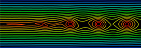
Kelvin-Helmholtz Instability Waves - Mathematica 4.2, C++, POV-Ray 3.6.1, 11/16/06
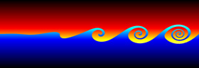
 Kelvin-Helmholtz instabilities are formed when one fluid layer is on top of another fluid layer moving with a different velocity. These instabilities take the form of small waves that can eventually grow into vortex rollers. This is a purely potential flow (irrotational) phenomenon. The following Mathematica code was adapted from Zheming Zheng’s Fortran program. It uses vortex blobs to simulate smooth rollers and periodic point vortices to simulate the far field. A simple predictor-corrector scheme is used to integrate the differential equations:
(* runtime: 9 minutes *) n = 40; dt = 0.05; L = 2Pi; gamma = L/n; rcore = 0.5; plist = Table[{x, 0.01 Sin[2Pi x/L]}, {x, 0, L(1 - 1/n), L/n}]; vcalc[plist_] := Table[Sum[{x, y} = plist[[j]] - plist[[i]]; gamma/(2Pi) Sum[If[i == j && k == 0, 0, r2 = (x + k L)^2 +y^2; {-y, x + k L}/r2(1 - Exp[-r2/rcore^2] - 1)], {k, -3, 3}] + If[i ==j, 0, gamma/(2L) {-Sinh[2Pi y/L], Sin[2Pi x/L]}/(Cosh[2Pi y/L] - Cos[2Pi x/L])], {j, 1, n}], {i, 1, n}]; Do[vlist = vcalc[plist]; vlist0 =vlist; vlist = vcalc[plist + dt vlist]; plist += dt(vlist0 + vlist)/2; ListPlot[plist, PlotJoined -> True, PlotRange -> {-2, 2}, AspectRatio -> Automatic], {i, 1, 400}]; |
 Here is some Mathematica code to plot streamlines assuming periodic point vortices:
(* runtime: 2 seconds *) Clear[psi]; psi[x_, y_] := Plus @@ Map[-gamma/(4 Pi) Re[Log[Cos[2Pi(x - #[[1]])/L] - Cosh[2Pi (y - #[[2]])/L]]] &, plist]; ContourPlot[psi[x, y], {x, 0, L}, {y, -L/3, L/3}, PlotRange -> All, ContourShading -> False, PlotPoints -> 20, AspectRatio -> Automatic] Link: Kelvin-Helmholtz waves in the clouds - Birmingham, Alabama |

 Here is another variation showing vortex pairing and pathlines.
Links Rayleigh-Taylor instability - instability between two fluids of different densities Droplet #7 - spherical Rayleigh-Taylor instability, by Mark Stock movie - famous experiment by Bernal |
Magnus Effect - C++, Mathematica 4.2, POV-Ray 3.6.1, 10/24/07
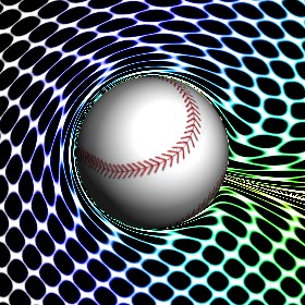


 A Curveball is a spinning ball that accelerates sideways due to the Magnus Effect. Here is some Mathematica code to plot the streamlines around a lifting cylinder, assuming inviscid incompressible potential flow (irrotational):
(* runtime: 0.3 second *) U = 1; gamma = 4; a = 1; w[z_] := U(z + a^2/z) + I gamma Log[z]/(2Pi); ContourPlot[Im[w[x + I y]], {x, -2, 2}, {y, -2, 2}, Contours -> Table[psi, {psi, -3, 3, 0.25}], PlotPoints -> 100, ContourShading -> False, AspectRatio -> Automatic] Here is some Mathematica code to plot the entrained fluid using the 4th order Runge-Kutta method: (* runtime: 17 seconds, increase n for better resolution *) Clear[v]; n = 40; U = 1; gamma = 4; a = 1; tmax = 5.0; dt = tmax/100; v[z_] := If[Abs[z] < 1, 0, Conjugate[U (1 - (a/z)^2) + I gamma/(2Pi z)]]; image = Table[z = x + I y; Do[k1 = dt v[z]; k2 = dt v[z + k1/2]; k3 = dt v[z + k2/2]; k4 =dt v[z + k3]; z -= (k1 + 2 k2 + 2 k3 + k4)/6, {t, tmax, 0, -dt}]; z, {y, -2, 2, 4.0/n}, {x, -2, 2, 4.0/n}]; ListDensityPlot[Map[Abs[Mod[#, 1]] &, image, {2}], Mesh -> False, Frame -> False, AspectRatio -> 1] Link: My Educational Project - some basic potential flows using Matlab and Mathematica |
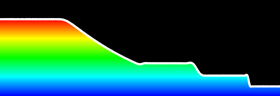
1D Shock Tube - Fortran 90, Mathematica 4.2, POV-Ray 3.6.1, 3/15/07

(* runtime: 5 seconds *) gamma = 1.4; R[W_] := Module[{}, rho = W[[All, 1]]; u = W[[All, 2]]/rho; p = (gamma - 1)(W[[All, 3]] - rho u^2/2); F = u W + Transpose[{Table[0, {n}], p, u p}]; h = Table[(F[[Min[n, i + 1]]] + F[[i]])/2, {i,1, n}]; Q = Table[h[[Max[i, 2]]] - h[[Max[i, 2] - 1]], {i, 1, n}]; nu = Table[i = Max[2, Min[n - 1, i]]; Abs[(p[[i + 1]] - 2p[[i]] + p[[i - 1]])/(p[[i + 1]] + 2p[[i]] + p[[i - 1]])], {i, 1, n}]; S = Table[Max[nu[[Min[n, i + 1]]], nu[[i]]], {i, 1, n}]; alpha1 = 1/2; beta1 = 1/4;alpha2 = alpha1; beta2 = beta1; epsilon2 = Map[Min[alpha1, alpha2#] &, S];epsilon4 = Map[Max[0, beta1 - beta2#] &, epsilon2];dW = Table[W[[Min[n - 1, i] + 1]] - W[[Min[n - 1, i]]], {i, 1, n}];dW3 = Table[i = Max[2, Min[n - 2, i]]; -W[[i - 1]] + 3W[[i]] - 3W[[i + 1]] + W[[i + 2]], {i, 1, n}];d = (epsilon2 dW - epsilon4 dW3)(Abs[u] + a); Dflux = Table[d[[Max[2, i]]] - d[[Max[2, i] - 1]], {i, 1, n}]; (Q - Dflux)/dx]; n = 50; dx = 1.0/n; a = 1.0; dt = dx/(1.0 + a); W = Table[{If[i > n/2, 0.125, 1], 0, If[i > n/2, 0.1, 1]/(gamma - 1)}, {i, 1, n}]; Do[W -= dt R[W - dt R[W - dt R[W]/4]/3]/2;ListPlot[W[[All, 1]], PlotJoined -> True,PlotRange -> {0, 1}, AxesLabel -> {"i", "rho"}], {t, 0, 100dt, dt}]; |


Jet - C++, 6/6/07
 This simulation is based on a simple method presented in this paper and sample C++ code by Jos Stam.
(* runtime: * seconds *) |
Schwarz-Christoffel Flow - C++, 11/*/07
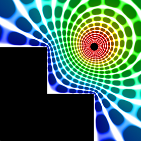
 Here is a potential flow field of a vortex near a flat wall mapped to stair steps using a Schwarz-Christoffel transformation. I got the inspiration for this stair step shape from Matthias Weber's website. Here is some Mathematica code:
(* runtime: 0.7 second *) Clear[z]; gamma = 1; z0 = 1 + I; z1 = I;z2 = 0; z3 = 1; zeta1 = -1; zeta2 = 0; zeta3 = 1; theta1 = 3Pi/2; theta2 = Pi/2; theta3 = 3Pi/2; z = z[zeta] /. DSolve[{z'[zeta] == K(zeta - zeta1)^(theta1/Pi - 1)(zeta - zeta2)^(theta2/Pi - 1)(zeta -zeta3)^(theta3/Pi - 1), z[zeta1] == z1}, z[zeta], zeta][[1]]; z = z /. K -> (K /. Solve[(z /. zeta -> zeta2) == z2, K][[1]]); zeta0 = zeta /. FindRoot[z == z0, {zeta, zeta2 + I}]; Z[w_] = z /. zeta -> (zeta /. Solve[w == (I gamma/(2Pi))(Log[zeta - zeta0] - Log[zeta - Conjugate[zeta0]]), zeta][[1]]); ToPoint[z_] := {Re[z], Im[z]}; grid = Table[ToPoint[Z[phi + I psi]], {phi, -1, 0, 0.05}, {psi, -1*^-6, -1, -0.02}]; Show[Graphics[{Map[Line, grid], Map[Line, Transpose[grid]]}, AspectRatio -> Automatic, PlotRange -> {{-1, 2}, {-1, 2}}]] Links My Educational Project - some basic potential flows using Matlab and Mathematica Schwarz-Christoffel Maps - nice plots by Matthias Weber used for minimal surfaces Schwarz-Christoffel Transformations - many examples by John Mathews |
Periodic Steady Vortices in a Stagnation Point Flow - C++, 11/17/07
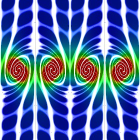
 I got the idea for this potential flow animation from this paper. The entrained fluid was integrated using the 4th order Runge-Kutta method.
 |
Vortices - Mathematica 4.2, C++, 10/31/06

 Here is another code to solve Euler’s equations (inviscid flow) and plot the pathlines. This method was adapted from Stephen Montgomery-Smith’s Euler2D program. The vortex effects are found using the Biot-Savart law and the differential equations are solved using the Adams Bashforth method. Click here to download some Matlab code for this. Shown below is some Mathematica code:
(* runtime: 19 seconds *) ToPoint[z_] := {Re[z], Im[z]};dt = 0.01; rcore = 0.1; dz0 = 0; Klist = {1, -1, 1, -1}; zlist = Join[{-1 - 0.5I, -1 + 0.5I, -0.5 - 0.5I, -0.5 + 0.5I}, Flatten[Table[x + I y, {x, -1, 1, 0.1}, {y, -1, 1, 0.1}], 1]]; paths = Map[# Table[1, {10}] &, zlist]; Do[dz = Map[Sum[zj = zlist[[j]]; If[# != zj, r2 = Abs[# - zj]^2; I Klist[[j]](zj - #)/r2 (1 -Exp[-r2/rcore^2]), 0], {j, 1, Length[Klist]}] &, zlist]; zlist += dt (1.5dz - 0.5dz0); dz0 = dz; paths = Table[Prepend[Delete[paths[[i]], -1], zlist[[i]]], {i, 1, Length[zlist]}];Show[Graphics[Map[Line[Map[ToPoint, #]] &, paths], PlotRange -> {{-1, 1}, {-1, 1}}, AspectRatio -> Automatic]], {85}]; Link: math paper by Stephen Montgomery-Smith, seems fairly advanced to me |
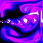
Ferrofluid - 4/6/05
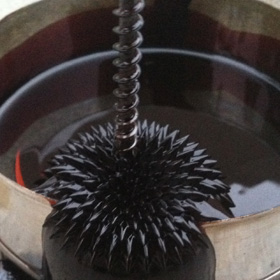 This magnetic fluid is great for visualizing magnetic fields (but it is very messy!). When you place a magnet under the fluid, it forms spikes called Rosensweig instability peaks. You can buy ferrofluid here.
Links Cymatic Ferrofluid - a clever way to fake Rosensweig instability peaks, by Robert Hodgin Magnetohydrodynamic Motor - how to make a simple magnetohydrodynamic propulsion device Ferrofluid Designs - beautiful designs made at MIT, see also their movie Morpho Tower - spiral Ferrofluid structure by Sachiko Kodama Ferrofluid Movies - at the University of Wisconsin, my favorites are the leaping ferrofluid and ferrofluid spikes Ferrofluid Photographs - Strange Matter exhibit |
Whirlpools - 3/16/08, 3/31/12
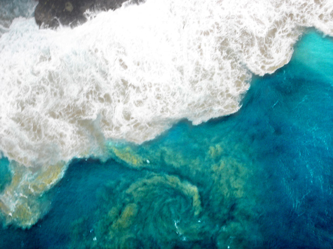
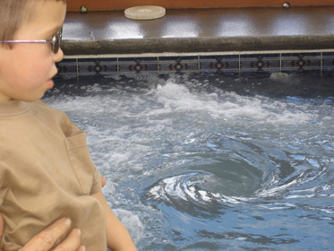 The left photo shows a giant whirlpool I saw below our helicopter during our Kauai helicopter tour. The right photo shows a small whirlpool we saw in a jacuzzi in Ecuador. See also my Maelstrom rendering.
Links Tourbillon barrage de la Rance - large whirlpool Fire Tornado - rarely seen, but fairly common during forest fires, here is another photo, here are videos from Honolulu and Brazil |
Smoke Ring - 10/13/07
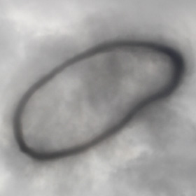 Here is a giant vortex ring of smoke from an explosion at the Miramar Air Show.
|
Supersonic Flow - CFL3D (Computational Fluids Laboratory 3D), Tecplot 360, 2/1/07
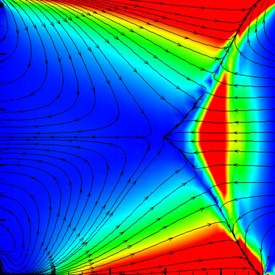
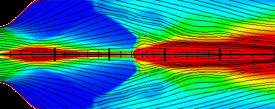 Here are some weird tests of CFL3D. The right image was my attempt to simulate shock diamonds. The color represents the Mach number.
 |
Channel Flow - Fluent 5.5.14, Gambit, Mathematica 4.2, 5/14/05

Fluid Motion Links
Gallery of Fluid Dynamics - excellent web site on fluid dynamics by Mark Cramer
Gallery of Fluid Motion - from the American Institute of Physics
Best Fluid Motion Pictures Named - National Geographic article
Oobleck - amazing non-Newtonian fluid that behaves like a solid when you move fast
Hydraulophone video - a hydraulophone works just like a flute except it uses water instead of air, the world's largest hydraulophone is at the Ontario Science Centre in Canada