


Here are some of my engineering simulations and related artwork.
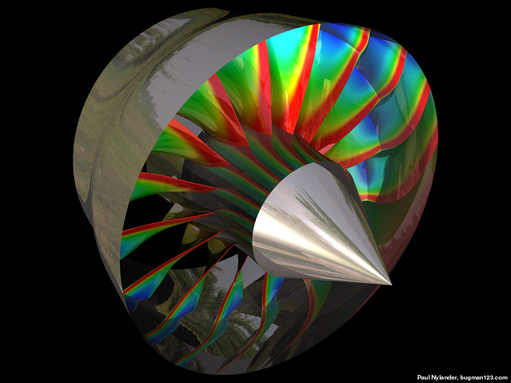
CFM56-5 Turbofan Jet Engine - drawn in AutoCAD 2000, AutoLisp, rendered in POV-Ray 3.6.1, 3/2/07
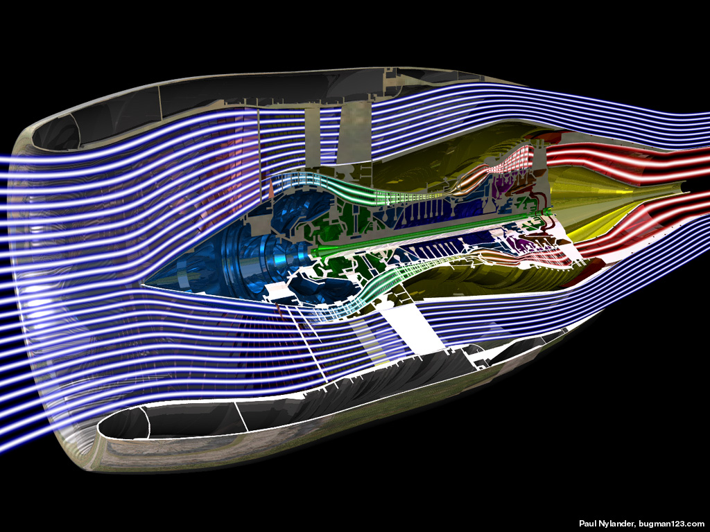
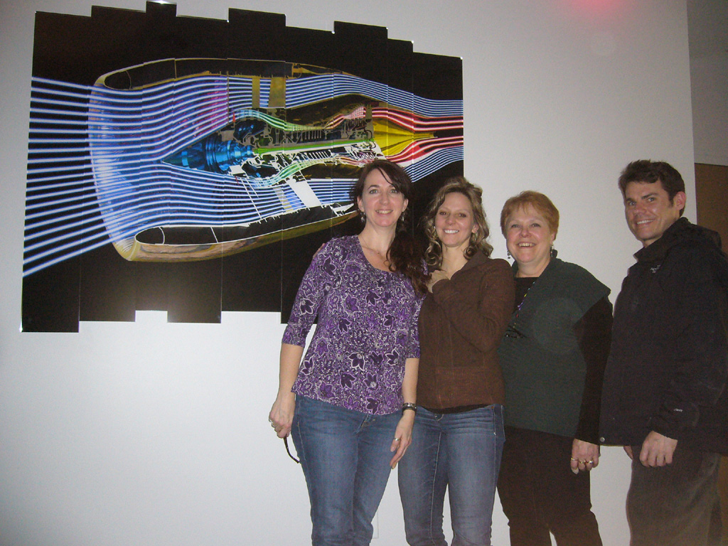
 This turbofan engine is used for the Airbus. I was inspired to create this 3D rendering from a schematic poster in our CFD lab. The streamlines shown here are just for visual effect. In reality, the streamlines would be turbulent. The blue streamlines show where cold air enters and bypasses the engine (turbofans typically have a high bypass ratio). Green streamlines are shown through the compressor stages. The red streamlines show where hot gas exits the burners and turbine stage. Click here to see a beautiful 5-foot acrylic display of this image, fabricated by Creative Encounters. You can purchase this as a poster here.
Links Geared TurboFan (GTF) - uses planetary gearing to reduce fan speed Working 3D Printed Turbofan Engine - designed by David Sheffler at University of Virginia |
3-Phase Brushless DC (BLDC) Motor - POV-Ray 3.6.1, 9/31/06
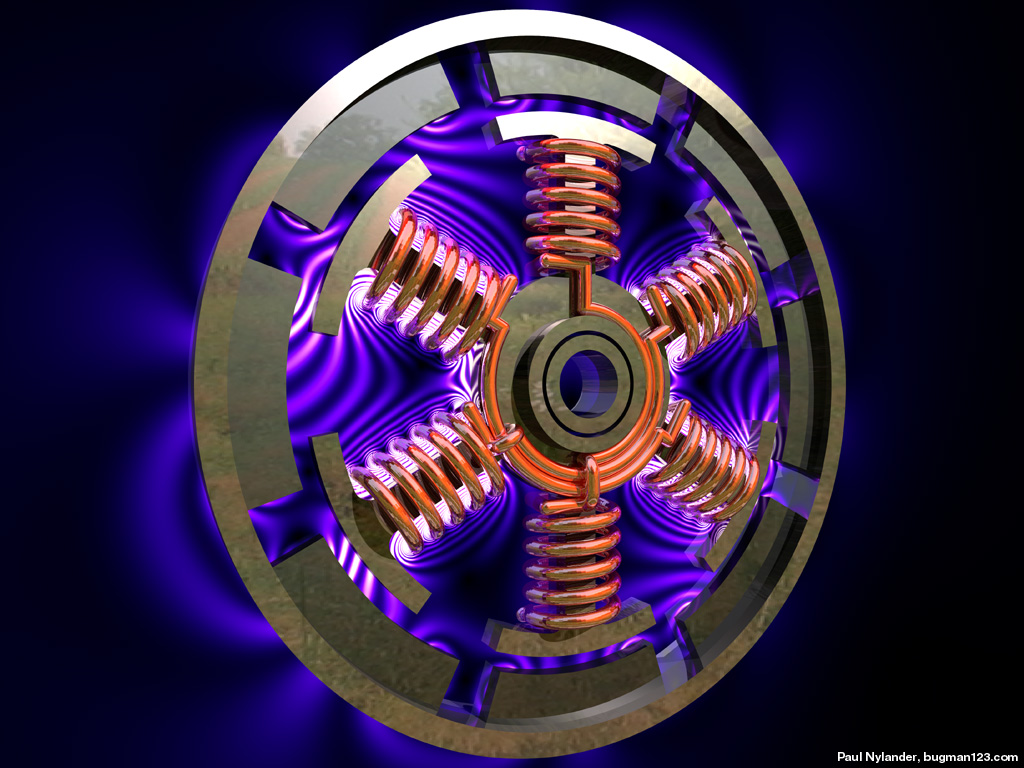
 Brushless motors are popular in model airplanes. This one has a 6 pole stator and an 8 pole rotor. The technique is very similar to that used in Maglev trains. This magnetic field was rendered using the same method as my magnetic field of a solenoid. See also my Tesla coil magnetic field.
Links Brushless Motor Schematics - by Gertjan Kool Finite Element Method Magnetics - free program by David Meeker The simplest motor of the world, Homopolar Motor, Motor Casero - YouTube videos demonstrating simple motors |
Inverse Kinematics Animation of Mladen Pejic's M-077 Mobile Support Platform (MSP)
LDraw, MLCad 2.11, L3P, POV-Ray 3.6.1, Mathematica 4.2, 6/8/06
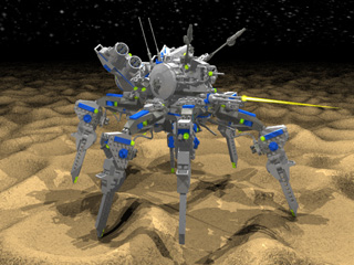
 The model I used for this animation is an original creation by Mladen Pejic, used with permission. All I have done here is animate it as an excercise in inverse kinematics. The walking animation uses the 6-legged “alternating tripod gait” which is common among insects. I animated the hoses under the legs using Rune Johansen’s inverse kinematics neck include file which uses a single cubic spline segment to approximately minimize the bending strain energy. (Note: if the movie doesn’t play right, you may need to save it to your computer first and then play it). The sound effects were combined together in Mathematica:
<< Miscellaneous`Audio`; AddSound[sound2_, sound1_,i_] := Module[{n1 = Length[sound1],n2 = Length[sound2]}, Join[Take[sound1, {1, Max[0, Min[n1, i - 1]]}], Take[sound1, {Max[1, Min[n1 + 1, i]], Max[0, Min[n1, i + n2 - 1]]}] + Take[sound2, {Max[1, Min[n2 + 1, 2 - i]], Max[0, Min[n2, n1 - i + 1]]}], Take[sound1, {Max[1, Min[n1 + 1, i + n2]], n1}]]]; sound = ReadSoundfile["C:/Sound.wav"][[1]]; rate = 44100; tmax = 1.0Length[sound]/rate; composition = Table[0, {Round[rate tmax]}]; Do[composition = AddSound[sound, composition, Round[rate t]], {t, 0, tmax, 0.25tmax}]; Export["C:/Composition.wav", ListPlay[composition, SampleRate -> rate]]; Links Robugtix - Adam Savage from MythBusters shows off his amazing Robugtix spider. Click here to see the spider dancing. Stompy - 2 ton hexapod robot, seeking funding on Kickstarter Biomimetics - my notes on insect flight LDraw - free Lego rendering program that works with POV-Ray Inverse Kinematics Tutorial - by Hugo Elias Spider Animation, Walking Animation, ArachnoBot - by Rune Johansen Hexapod Robot CNC Router - sculpting 3D face Timberjack Walking Machine Do You Remember Macross - Robotech animation by Tipatat Chennavasin |
Finite Element Method (FEM) Solution to Poisson’s equation on Triangular Mesh
solved in Mathematica 4.2, 5/24/06; mesh generated with Gmsh (old version: Matlab and DistMesh)
 Here is some Mathematica code to solve Poisson’s equation on an unstructured grid of triangular elements using the Finite Element Method (FEM): (* runtime: 0.02 second *) n = 10; nodes = Flatten[Table[{x, y}, {y, -1, 1, 2.0/(n - 1)}, {x, -1, 1, 2.0/(n - 1)}], 1]; elems = Flatten[Table[i + {{0, 1, n}, {1, n + 1, n}} + (j - 1) n, {j, 1, n - 1}, {i, 1, n - 1}], 2]; nnode = Length[nodes]; nelem = Length[elems]; fixed = Map[Position[nodes, #][[1, 1]] &, Select[nodes, Max[Abs[#]] == 1 &]]; free = Complement[Range[nnode], fixed]; Kglobal = Table[0, {nnode}, {nnode}]; F = phi = Table[0, {nnode}]; Scan[(xy =Join[Transpose[nodes[[#]]], {{1, 1, 1}}];deta = Inverse[xy][[All, {1, 2}]]; Kglobal[[#, #]] +=Det[xy]deta.Transpose[deta]/2; F[[#]] += Det[xy]/6) &, elems]; phi[[free]] = LinearSolve[Kglobal[[free, free]], F[[free]]]; Mean[x_] := Plus @@ x/Length[x]; PlotColor[x_] := Hue[2(1 - x)/3]; Show[Graphics[Table[{PlotColor[Mean[phi[[elems[[i]]]]]/Max[phi]], Polygon[nodes[[elems[[i]]]]]}, {i,1, nelem}], AspectRatio -> 1]] Here is some Mathematica code for an interpolated plot: (* runtime: 8 seconds *) n = 275; x1 = y1 = -1; x2 = y2 = 1; image = Table[0, {n}, {n}]; xIntersect[{{x1_, y1_}, {x2_, y2_}}] := If[y1 == y2, Infinity, x1 + (y - y1)(x2 - x1)/(y2 - y1)]; Scan[(plist = nodes[[#]]; xlist = nodes[[#, 1]]; ylist = nodes[[#, 2]]; p1 = plist[[1]]; {dx2, dy2} = plist[[2]] - p1; {dx3, dy3} = plist[[3]] - p1; Do[y = y1 + (y2 - y1)(i - 1)/(n - 1); {xa, xb,xc} = Map[xIntersect, Partition[Sort[plist, #1[[2]] < #2[[2]] &], 2, 1, 1]]; jlist = Round[n({xc, If[Abs[xb - xc] < Abs[xa - xc], xb, xa]} - x1)/(x2 - x1)]; If[jlist =!= {}, Do[x = x1 + (x2 - x1)(j - 1)/(n - 1); {xi, eta} = ((x - p1[[1]]){dy3, -dy2} + (y - p1[[2]]){-dx3, dx2})/(dx2 dy3 - dx3 dy2); image[[i, j]] = phi[[#]].{1 - xi - eta, xi, eta}, {j, Max[1, Min[jlist]], Min[n, Max[jlist]]}]], {i, Max[1, Round[n(Min[ylist] - y1)/(y2 - y1)]], Min[n, Round[n(Max[ylist] - y1)/(y2 - y1)]]}]) &, elems]; ListDensityPlot[image, Mesh -> False, Frame -> False, ColorFunction -> PlotColor, Epilog -> Map[{Line[Map[({x, y} = nodes[[#, {1, 2}]]; n{(x - x1)/(x2 -x1), (y - y1)/(y2 - y1)}) &, #]]} &, elems]] |
 Here is some Mathematica code to solve Poisson’s equation on an unstructured grid of quadrilateral elements:
(* runtime: 0.05 second *) n = 10; nodes = Flatten[Table[{x, y}, {x, -1, 1,2.0/(n - 1)}, {y, -1, 1, 2.0/(n - 1)}], 1]; nnode = Length[nodes]; elems =Flatten[Table[{i, i + 1, i + n + 1, i + n} + (j - 1) n, {j, 1, n - 1}, {i, 1, n - 1}], 1]; nelem = Length[elems]; fixed = Map[Position[nodes, #][[1, 1]] &, Select[nodes, Max[Abs[#]] == 1 &]]; free = Complement[Range[nnode], fixed]; Kglobal = Table[0, {nnode}, {nnode}]; F = phi = Table[0, {nnode}]; Scan[(plist = nodes[[#]]; dphi = {plist[[2]] - plist[[1]],plist[[4]] - plist[[1]]}; B = Inverse[Transpose[dphi].dphi]; C1 = {{2, -2}, {-2, 2}}B[[1, 1]] + {{3, 0}, {0, -3}}B[[1, 2]] + {{2, 1}, {1,2}}B[[2, 2]];C2 = {{-1, 1}, {1, -1}}B[[1, 1]] + {{-3, 0}, {0, 3}} B[[1, 2]] + {{-1, -2}, {-2, -1}}B[[2, 2]]; Kglobal[[#, #]] += Det[dphi]Join[Thread[Join[C1, C2]], Thread[Join[C2, C1]]]/6; F[[#]] += Det[Join[{{1, 1, 1}}, Transpose[nodes[[#[[{1, 2, 3}]], {1, 2}]]]]]/4) &, elems]; phi[[free]] = LinearSolve[Kglobal[[free, free]], F[[free]]]; Mean[x_] := Plus @@ x/Length[x]; PlotColor[x_] := Hue[2(1 - x)/3]; Show[Graphics[Table[{PlotColor[Mean[phi[[elems[[i]]]]]/Max[phi]], Polygon[nodes[[elems[[i]]]]]}, {i, 1, nelem}], AspectRatio -> 1]] Links FEM_50 - simple Matlab Poisson solver for quads and triangles FEM Poisson - paper by Nasser Abbasi Poisson solver - simple finite volume C code by Jeroen Valk |
Finite Element Analysis (FEA) - AutoCAD 2000, AutoLisp, Mathematica 4.2, 5/26/06
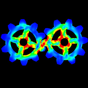
 Here we see the deformation and stress distribution between two gears where the left gear is fixed but the right gear has an applied torque. This was solved using Finite Element Analysis (FEA) to solve the linear elasticity equations for an unstructured grid of quadrilateral elements. The color represents the equivalent (Von Mises) stress calculated from the Cauchy stress tensor. Here is some Mathematica code:
(* runtime: 1.5 second *) n = 36; dtheta = 2Pi/n; nodes = Flatten[Table[r{Sin[theta], Cos[theta]}, {r, 1, 2, 0.25}, {theta, 0, 2Pi - dtheta, dtheta}], 1]; elems = Flatten[Table[n j + Append[Table[i + {0, 1, n + 1, n}, {i, 1, n - 1}], {1, n + 1, 2n, n}], {j, 0, 3}], 1]; nnode = Length[nodes]; nelem = Length[elems]; i = 3n/2 + 1; fixed = {{i - 1, "x"}, {i, "x"}, {i, "y"}, {i + 1, "x"}}; loads = {{n + 1, {0, -200}}}; Dkl := 0.25{{-1 + y, 1 - y, 1 + y, -1 - y}, {-1 + x, -1 - x, 1 + x, 1 - x}}; Dkm = 0.25{{-1, 1, 1, -1}, {-1, -1, 1, 1}}; e = 1500; nu = 0.3; Epss = {{1, nu, 0}, {nu, 1, 0}, {0, 0, (1 - nu)/2}}e/(1 - nu^2); thk = 1; Kglobal = Table[0, {2nnode}, {2nnode}]; Scan[(element = #; enodes = nodes[[element]]; Klocal = Table[0, {8}, {8}]; Kee = Table[0, {4}, {4}]; Kre = Table[0, {8}, {4}]; Scan[({x, y} = #/Sqrt[3]; t = Inverse[Dkl.enodes].Dkl; strain = {{t[[1, 1]], 0, t[[1, 2]], 0, t[[1, 3]], 0, t[[1, 4]], 0}, {0, t[[2, 1]], 0, t[[2, 2]], 0, t[[2, 3]], 0, t[[2, 4]]}, {t[[2, 1]], t[[1, 1]], t[[2, 2]], t[[1, 2]], t[[2, 3]], t[[1, 3]], t[[2, 4]], t[[1, 4]]}}; ttm = -2Inverse[Dkm.enodes].{{x, 0}, {0, y}}; ct = {{ttm[[1,1]], 0, ttm[[1, 2]], 0}, {0, ttm[[2, 1]], 0, ttm[[2, 2]]}, {ttm[[2, 1]], ttm[[1, 1]], ttm[[2, 2]], ttm[[1, 2]]}}Det[Dkm.enodes]/Det[Dkl.enodes]; Dj = thk Abs[Det[Dkl.enodes]]; Klocal += Transpose[strain].(Epss.strain) Dj; Kee += Transpose[ct].(Epss.ct) Dj; Kre += Transpose[strain].(Epss.ct) Dj) &, {{-1, -1}, {1, -1}, {1, 1}, {-1, 1}}];Klocal -= Kre.Inverse[Kee].Transpose[Kre];Do[Kglobal[[2element[[i]] - di, 2element[[j]] - dj]] += Klocal[[2i -di, 2j - dj]], {di, 0, 1}, {dj, 0, 1}, {i, 1, 4}, {j, 1,4}]) &, elems]; Scan[(i = 2#[[1]] - If[#[[2]] == "x", 1, 0]; Kglobal[[i, i]] *= 10^6) &, fixed]; paload = Table[0, {2nnode}]; Scan[(paload[[2#[[1]] - {1, 0}]] = #[[2]]) &, loads]; del = Partition[LinearSolve[Kglobal, paload], 2]; Do[nodes2 = nodes + scale del; Show[Graphics[Map[Line[nodes2[[#]]] &, elems], AspectRatio -> Automatic]], {scale, 0, 1, 0.1}]; |
 Links
LinksGears - nice FEA animation by Noran Engineering, Inc. (where I used to work) Gears in Oil - cool fluid-structure interaction simulation by * Introduction to Finite Element Methods - online book by Carlos Felippa Mathematica FEA - code for 2D beam using quad elements, by Chee Kiang Yew Mini-FEA - simple Java applet IMTEK Mathematica Supplement - free FEA and meshing packages Rubber Membrane - interesting animation of buckling behavior Physica - has the ability to do “MultiPhysics” (for example, fluid-structure interaction) Real-Time FEA - cool Java applet for 3D beam by Matthias M�ller-Fischer AceFEM - FEA environment for Mathematica |
St. Louis Arch - calculated in Mathematica 4.2, rendered in POV-Ray 3.6.1, 10/6/06
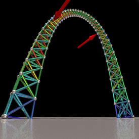

 The St. Louis Arch is shaped like an upside-down catenary for maximum support. This image was simulated as a system of linear static 1D beam elements. The non-linear animation on the right was simulated using many small linear solutions. Here is some Mathematica code:
(* runtime: 0.25 second *) x0 = 299.2239; h = 625.0925; a = 118.6261; n = 20; EA = 25000.0; nodes = Flatten[Table[z = a(Cosh[x0/a] - Cosh[x/a]); r = 54 - 37z/h; Table[{x, 0, z} + r{-Tanh[x/a]Cos[theta], Sin[theta], -Sech[x/a]Cos[theta]}, {theta, 0, 4Pi/3, 2Pi/3}], {x, -x0, x0, 2x0/n}], 1]; elems = Flatten[Table[Join[{{1, 2}, {2, 3}, {3, 1}}, If[i < n, {{1, 4}, {2, 5}, {3, 6}, {1, 5}, {2, 6}, {3, 4}}, {}]] + 3i, {i, 0, n}], 1]; fixed = Join[{1, 2, 3}, nnode - {2, 1, 0}]; nnode = Length[nodes]; nelem = Length[elems]; nfixed = Length[fixed]; free = Complement[Range[nnode], fixed]; A = Map[({i1, i2} = #; del = nodes[[i2]] - nodes[[i1]]; del /= del.del; Flatten[Table[If[i == i1, -1, If[i == i2, 1, 0]]del, {i, 1, nnode}][[free]]]) &, elems]; Kglobal = EA Transpose[A].A; Q = Table[{0, 0, 0}, {nnode}]; Q[[Ceiling[nnode/2]]] = {0, 1, 0}; q = Table[{0, 0, 0}, {nnode}]; q[[free]] =Partition[LinearSolve[Kglobal, Flatten[Q[[free]]]], 3]; e = Map[({i1, i2} = #; q[[i1]] - q[[i2]]) &, elems]; s = Map[Sqrt[#.#] &, e]; smax = Max[s]; Do[Show[Graphics3D[Table[elem = elems[[i]]; {Hue[2(1 - scale s[[i]]/smax)/3], Line[nodes[[elem]] + scale q[[elem]]]}, {i, 1, nelem}]]], {scale, 0, 1, 0.1}]; In case you're wondering how to create your own LinearSolve function, one method you can use (albeit innefficient) is Gaussian elimination with partial pivoting and back substitution (a more efficient approach would be to a sparse matrix solver): LinearSolve[A_, x_] := Module[{n = Length[A], i = 1, j = 1, imax, B}, B = Table[Append[A[[i]], x[[i]]], {i, 1, n}]; While[i <= n && j <= n + 1,imax = i; Do[If[Abs[B[[k, j]]] > Abs[B[[imax, j]]], imax = k], {k, i + 1, n}]; If[B[[imax, j]] != 0.0, {B[[i]], B[[imax]]} = {B[[imax]], B[[i]]}; B[[i]] /= B[[i, j]]; Do[B[[u]] -= B[[u, j]] B[[i]], {u, i + 1, n}]; i++]; j++]; Do[B[[i, n + 1]] = (B[[i, n + 1]] - Sum[B[[i, j]]B[[j, n + 1]], {j, i + 1, n}])/B[[i, i]], {i, n - 1, 1, -1}]; B[[All, n + 1]]]; Links Deflecting Arch - Mathematica animation by L. Zamiatina Space Truss - Mathematica notebook by Carlos Felippa Sim-POV - mechanics simulations for POV-Ray by Christoph Hormann |
Expanding Dodecahedron - POV-Ray 3.6.1, 2/1/07
 This dodecahedron unfolds and expands by a factor of 2.61803 (the golden ratio plus one). Perhaps it would be possible to construct something similar to this. I think it would make an interesting display for a children’s science museum.
Links Hoberman Sphere - popular icosidodecahedron toy that expands Switch Kick - clever toy ball that turns inside-out Juno's Spinner - expanding spheres with rotating faces, by Junichi Yananose |
Radial Engine - POV-Ray 3.6.1
 under construction
Links Radial Engine Mechanicard - by Brad Litwin |
Four-Stroke Otto Cycle - POV-Ray 3.6.1
 under construction
Links Wankel Engine - a unique engine Engine Assembly - nice FEA animation by Noran Engineering, Inc. (I used to work here), based on this model V8 Model - free Solidworks model from 3D ContentCentral |
Torque Converter - POV-Ray 3.6.1
 under construction
 |
Helicopter Rotor
 under construction. See collective cyclic pitch.
Links Atlas Human-Powered Helicopter - by Todd Reichert and Cameron Robertson Palmsize Micro Copter - amazing tiny toy largest helicopters in the world Remote Control Dragonfly - video Tip-Jet Rotors - jet engines on tips of helicopter blades Remote Control V-22 Osprey - YouTube video, with jet-engine Mesicopter - very small helicopter proposed for Mars exporation, by Ilan Kroo and Friedrich Prinz Pixelito - 6.9 gram helicopter Micro Coaxial Rotorcraft - by Felipe Bohorquez, here is a video and an explanation Chaos maneuver - pitch, roll, yaw Flying Ball JSDF Floating Orb Robot - includes video camera, created by the Japanese army Six-Inch MAV - can be launched by throwing it like a frisbee, by Michael Nechyba |
Turbofan Blades - rendered in POV-Ray 3.6.1, 3/1/07
 I rendered this from a turbofan blade model that was studied in our CFD lab.
Links GE90-115B Gas Turbine - world’s most powerful jet engine EngineSim - Java applet for learning about jet engines, here is another one M400 Skycar - flying car, Vertical Take-Off and Landing (VTOL), be sure to see the interview with Dr. Moller ThrustSSC - first supersonic land speed record Miniature Harrier - amazing remote control AVAB Harrier with Pegasus engine by Ewald Schuster Jet-Powered Go Kart - 100 mph small jet engines - homemade, engine, model, red hot afterburner test remote control jet - 200 mph, here’s another one that goes 270 mph Chrysler Turbine Car Enercon E-126 - world's largest wind turbine World's Largest Tidal Farm - by OpenHydro |
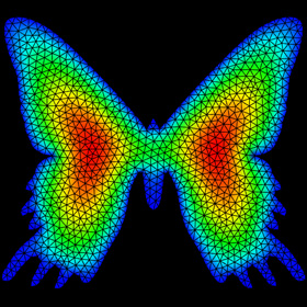
Torsion Beam - calculated in Mathematica 4.2, rendered in POV-Ray 3.6.1, 5/3/06
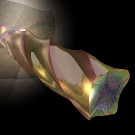
 Here is an exaggerated example of a beam being twisted. The following Mathematica code is based on Stephen Timoshenko’s analytical solution. The color represents the equivalent (Von Mises) stress where red is high stress and blue is low stress.
(* runtime: 12 seconds *) Clear[f, x, y]; a = b = 2.0; L = 10; T = G = 1; J = 16/3a^3b(1 - 196a/(b Pi^5)Sum[n^-5Tanh[n Pi b/(2a)], {n, 1, 200, 2}]); k = T/(G J); phi = 32G k a/Pi^3Sum[1/n^3(-1)^((n - 1)/2)(1 - Cosh[n Pi y/(2a)]/Cosh[n Pi b/(2a)])Cos[n Pi x/(2a)], {n, 1, 10, 2}]; tauyz = -D[phi, x]; tauxz = D[phi, y]; tauxy = sx = sy = sz = 0; f[x_, y_, z_] := Module[{}, {s1, s2, s3} = Eigenvalues[{{sx, tauxy, tauxz}, {tauxy, sy, tauyz}, {tauxz, tauyz, sz}}]; sv = Sqrt[((s1 - s2)^2 + (s2 - s3)^2 + (s3 - s1)^2)/2]; {x - k z y, y + k z x, z, {EdgeForm[], SurfaceColor[Hue[2(1 - sv/0.029)/3]]}}]; << Graphics`Master`; DisplayTogether[Map[{ParametricPlot3D[f[#a/2, y, z], {y, -b/2, b/2}, {z, 0,L}, Compiled -> False], ParametricPlot3D[f[x, #b/2, z], {x, -a/2, a/2}, {z, 0, L}, Compiled -> False]} &, {-1, 1}], ParametricPlot3D[f[x, y, L], {x, -a/2, a/2}, {y, -b/2, b/2}, Compiled -> False]]; Links Computer Modeling - class notes by Nasser Abbasi Torsional Analysis - part of the Structural Mechanics Mathematica package |
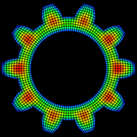
Solution to Poisson’s equation on Structured Grid - calculated in GridPro, rendered in POV-Ray 3.6.1, 10/5/06
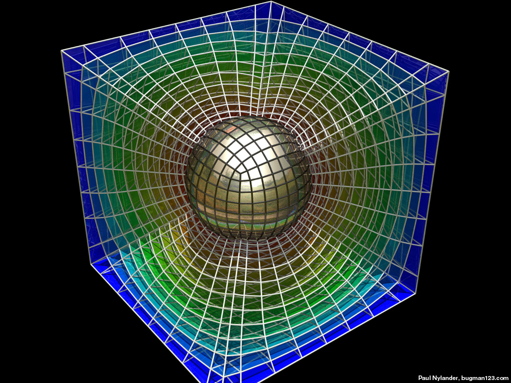
 Here is a structured hexahedral grid. Structured grids are often used when solving numerical simulations, especially in CFD simulations. These grids can usally solve problems with high speed and accuracy, but they can be challenging to work with when modelling irregular shapes. This mesh was generated using GridPro. GridPro optimizes the grid spacing by placing gridpoints along isosurfaces of the solution to the Poisson equation.
 |
Unstructured Tetrahedral Meshed Sphere - DistMesh, Matlab, POV-Ray 3.6.1, 6/12/06
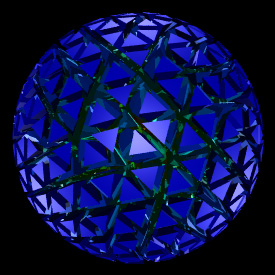
 Here is an unstructured tetrahedral meshed sphere. Unstructured grids are also often used for solving numerical simulations, especially FEA simulations. These grids can be easier for modelling irregular shapes than structured grids, but sometimes they take longer to solve and are less accurate.
Links Mesh Generation - interesting paper by Per-Olof Persson polyhedral mesh - Fluent's unstructured mesh for complex geometry Free Mesh Generators - click here for a complete list: CUBIT (not free) - impressive hexahedral mesh generator |
Cube - POV-Ray 3.6.1, 1/31/07
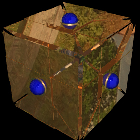
 This is a cube that expands by a factor of 3. I think it would be difficult to contruct something similar to this.
Link: Atomium - 335 foot tall cube building in Brussels built in 1958 |
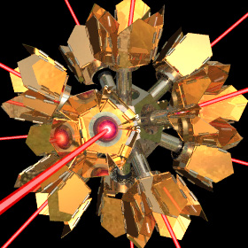
Inverse Kinematics Animation of Mladen Pejic's “Valour” Advanced Gunship - LDraw, MLCad 2.11, L3P, POV-Ray 3.6.1, 6/15/06
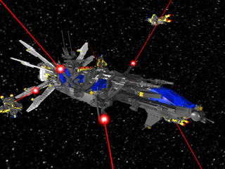
 The model in this animation is an original creation by Mladen Pejic, used with permission. All I have done here is animate it as an excercise in inverse kinematics. The ship is doing laser target practice in this animation.
 |
Folding Wing Aircraft
calculated in CFL3D (Computational Fluids Laboratory 3D), rendered in POV-Ray 3.6.1, 11/3/06
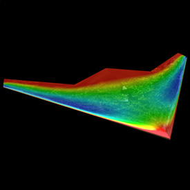
 This is a preliminary test of a proposed project to simulate the wing fluttering of an aircraft with folding wings. This was solved using the finite volume method for 3D, steady, compressible, viscous, laminar flow on a curvilinear grid. This image shows the pressure distribution over the wings.
Links papers - wing flutter and gridless methods by Feng Liu |
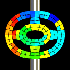
Simply Loaded Beam - Patran, Nastran (NASA Structural Analysis), 9/28/06
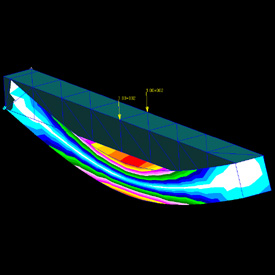 Nastran was originally created by NASA but now other companies are distributing it. This was a simple class assignment. I’m planning to post a more interesting picture here later.
 |
Biomimetics Links
Biomimetics is the study of biological mechanisms in order to engineer machines that can mimic them.
SmartBird - by Festo Company
RoboCup - International robotic soccer competitions. Their goal is to build robots that can defeat champion human soccer players by the year 2050. It looks like they still have a way to go. See also RoboGames.
Hanson Robotics - most realistic looking humanoid robots by David Hanson
Bionic Dolphin - this submarine is too buoyant to go underwater, but when it goes fast enough, its "flippers" work like upside-down airplane "wings" to force it under water.
Luke Arm - prosthetic arm by Dean Kamen, the inventor of Segway
Airic's Arm - bionic arm operated by "Fluidic Muscles"
more biomimetics links: Air-Ray (very cool flying manta ray), Aqua-Ray (underwater manta ray), Snake Robot (see video and sidewinding snake), robotic dragonfly toy, NASA's robotic serpent, BigDog, Stickybot (Gecko), RoboPike, robotic caterpillar, RoboSnail, robotic mule, RoboStrider, RoboRoach hexapod, robotic dolphin, robotic penguin, RoboLobster
Other Engineering Links
Breaking the Sound Barrier Underwater - uses Supercavitation to create a bubble
The Future of Things (TFOT) - tons of high-tech gadgets
Wally Wallington - this guy is single-handedly building his own Stonehenge using only his own strength
Freedom Ship - proposed ship, 3 million tons, 4500 feet long
Habbakuk - proposed Pykrete aircraft carrier during World War II, 2 million tons, 2000 feet long
Space Elevator - made from carbon nanotubes
Microsubmarine
PowerLabs (Sam Barros) - impressive projects, see the rail gun, jet turbine, and high speed CD-Rom experiments
Motorized Surfboard
Flexinol - wires that electronically contract like muscles, sample kit was $30 last time I checked
Air Muscle - interesting actuator
Holographic Flat Panel - uses parallax to create a 3D effect, no glasses required
World’s Smallest Internal Combustion Engine
Manned-Cloud - flying hotel that will go around the world in 3 days
wind-powered art sculpture - weighs nearly 3 tons with living quarters inside, by Theo Jansen
Cloud-busting - how to make it rain using liquid nitrogen
Architecture Links
Extreme Engineering - interesting Discovery web site on ambitious architectural plans
Skyscraper Page - over 16000 scale drawings of famous buildings
Floating Observatories - unusual tower in Taiwan with floating elevators
Ark Hotel - floating hotel
The Palm Island - man-made island in Dubai
ETFE (Ethylene Tetrafluoroethylene) - new high strength insulating plastic, check out this amazing picture